How to Instantly Remove Duplicates in Excel

Ever stared at a sprawling Excel spreadsheet, knowing there are duplicate entries lurking, silently skewing your reports, inflating your numbers, and just generally making a mess? You’re not alone. Duplicate data is a common headache for anyone managing information, from student project lists to enterprise sales figures. Manually sifting through thousands of rows to find and delete them is not just time-consuming; it’s an exercise in frustration. But what if I told you that Excel has powerful, built-in features that can help you instantly remove duplicates in Excel with just a few clicks?

At AskByteWise.com, our mission is “Making Complex Tech Simple.” Today, as Noah Evans, your guide through the world of data, I’m going to show you exactly how to take back control of your spreadsheets. This comprehensive guide will transform you from a duplicate-data victim into a data-cleaning wizard, ensuring your information is pristine, accurate, and ready for analysis. Let’s dive in and learn how to instantly remove duplicates in Excel!

Why Duplicates Are a Data Nightmare (and How Excel Saves the Day)

Before we get to the “how-to,” let’s quickly underscore why removing duplicates is so crucial. Imagine you’re tracking customer orders, and one customer accidentally placed the same order twice, or their details were entered slightly differently across two systems. If you don’t catch these duplicates:

Inaccurate Reporting: Your sales figures might be inflated, your customer count skewed, or your inventory levels misrepresented.
Wasted Resources: Sending follow-up emails to the same customer twice, shipping duplicate products, or allocating resources based on incorrect data.
Poor Decision-Making: All business decisions are only as good as the data they’re based on. Duplicate data leads to flawed insights.
Credibility Loss: Presenting reports with obvious duplicate entries can undermine your professionalism and the trust placed in your data.

Excel understands these challenges, and that’s why it offers remarkably efficient tools to help you identify and remove duplicates in Excel without breaking a sweat.

The Easiest Way: Using Excel’s Built-In “Remove Duplicates” Feature

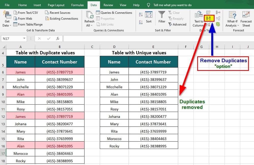
When you need to instantly remove duplicates in Excel from your dataset, Excel’s dedicated “Remove Duplicates” feature is your go-to solution. It’s fast, effective, and handles entire rows, ensuring your remaining data stays intact and consistent.

Step-by-Step Guide to Using “Remove Duplicates”

Follow these simple steps to clean your data like a pro:

Select Your Data Range:
- The most critical first step is to select all the data you want to check for duplicates. If you only select a single column, Excel will only check that column for duplicates and delete entire rows based on those findings, which might lead to unintended data loss in other columns.
- To select your entire dataset, click on any cell within your data and press Ctrl + A (Windows) or Cmd + A (Mac). If your data is contiguous, this will select the entire range. Alternatively, click and drag your mouse to highlight all relevant cells.
- Important Note: Make sure to include any header row in your selection if you have one. Excel uses headers to help you identify columns during the removal process.
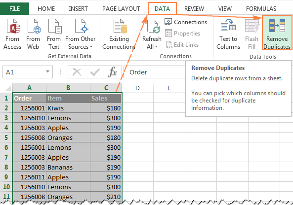
Navigate to the Data Tab:
- Once your data is selected, look for the Data tab in Excel’s ribbon interface at the top of your screen. Click on it.
Click “Remove Duplicates”:
- Within the Data tab, in the “Data Tools” group, you’ll find an icon labeled Remove Duplicates. It typically looks like a table with a red “X” next to one of the rows. Click this icon.
Configure the “Remove Duplicates” Dialog Box:
- A dialog box will appear. This is where you tell Excel which columns to consider when looking for duplicates.
- “My data has headers” checkbox: If your selected data includes a header row (highly recommended!), make sure this box is checked. This tells Excel to use the column names (like “Customer Name,” “Product ID”) instead of generic “Column A,” “Column B,” etc., making the process much clearer.
- Select Columns: Below the header checkbox, you’ll see a list of all columns in your selected data.
  - To instantly remove duplicates in Excel based on all columns (meaning a row is a duplicate only if every single cell in that row matches another row exactly), simply ensure all columns are checked (the default).
  - If you want to remove duplicates based on a specific subset of columns (e.g., remove duplicate customer names, even if their order date is different), uncheck the columns that shouldn’t be considered when determining a duplicate. For example, if you want to find rows where the “Product ID” and “Order Date” are the same, but the “Quantity” might differ, you’d only check “Product ID” and “Order Date.”
Confirm and Execute:
- After you’ve made your column selections, click OK.
- Excel will quickly process your data and then display a message box telling you how many duplicate values were found and removed, and how many unique values remain.
- Click OK to close this message.
Review Your Cleaned Data:
- Your spreadsheet will now only contain unique rows based on your specified criteria. Scroll through and ensure the results are as expected.

Important Considerations for the “Remove Duplicates” Feature

Case Sensitivity: By default, Excel’s “Remove Duplicates” feature is not case-sensitive. This means “Apple” and “apple” will be treated as the same value. If case sensitivity is critical for your data (e.g., product codes), you might need an alternative approach like using formulas or adjusting your data beforehand.
Original Data Loss: When you use “Remove Duplicates,” the duplicate rows are permanently deleted. There is no “undo” button for this specific action after you’ve saved and closed the file. Always back up your data before using this feature! A simple copy-paste of your sheet into a new tab or workbook can save you a lot of heartache.
Partial vs. Exact Matches: Understand that Excel only removes exact duplicates based on the columns you select. Minor differences, like an extra space, a comma in a different place, or a slightly different spelling (“AskByteWise” vs. “Ask ByteWise”), will be treated as unique entries.
Hidden Rows/Columns: If you have hidden rows or columns within your selected range, the “Remove Duplicates” feature will still include them in its analysis and potentially remove them. Unhide all rows and columns before starting if you’re unsure.

Tip: If you only want to see duplicates without deleting them, or need more advanced filtering, Excel offers other powerful tools, which we’ll explore next.

Beyond Simple Removal: Identifying Duplicates Without Deleting Them

Sometimes, you don’t want to simply delete duplicates. You might need to review them first, understand why they are duplicates, or choose which instance to keep. For these scenarios, Conditional Formatting is your best friend.

Using Conditional Formatting to Highlight Duplicates

Conditional Formatting allows you to visually identify duplicates, giving you the power to inspect and decide what action to take.

Select the Data Range:
- Highlight the column(s) or the entire data range where you want to find duplicate values. If you want to highlight duplicate entries across multiple columns (i.e., highlight a row if a combination of values in that row is duplicated), select all relevant columns.
Go to the Home Tab:
- Click on the Home tab in the Excel ribbon.
Access Conditional Formatting:
- In the “Styles” group, click on Conditional Formatting.
Select “Highlight Cell Rules” and “Duplicate Values”:
- From the dropdown menu, hover over Highlight Cell Rules, then click Duplicate Values….
Choose Your Formatting:
- A dialog box will appear, allowing you to choose how you want the duplicate values to be formatted (e.g., “Light Red Fill with Dark Red Text,” “Yellow Fill,” etc.). You can also choose “Custom Format…” for more options.
- Make sure “Duplicate” is selected in the first dropdown menu (it’s usually the default).
Apply and Review:
- Click OK. Instantly, all duplicate values in your selected range will be highlighted according to your chosen format.

Now, you can visually scan your data, review the highlighted cells, and make informed decisions. You might decide to manually edit some, delete others, or use the “Remove Duplicates” feature on a subset of the data after your review. This method is incredibly helpful for understanding your data before making permanent changes.

Advanced Techniques: Using Formulas to Identify and Filter Duplicates

While Excel’s built-in features are excellent, using formulas gives you even more control and flexibility, especially if you need to perform calculations based on duplicate status or want to identify only the first or last instance of a unique record. This is where your inner data analyst truly shines, and it’s a powerful way to instantly remove duplicates in Excel or just mark them for further processing.

The COUNTIF Function for Duplicate Identification

The COUNTIF function is a staple in any data analyst’s toolkit. It counts the number of cells within a range that meet a specified criterion. We can leverage this to count how many times each value appears, thus identifying duplicates.

How it works: You create a formula that counts how many times the value in the current cell appears in the entire column. If the count is greater than 1, it’s a duplicate.

Let’s assume your data is in Column A, starting from cell A2.

Insert a New Column: Add a new column next to your data (e.g., Column B) and label it “Duplicate Status” or “Count.”
Enter the COUNTIF Formula: In cell B2 (assuming your data starts in A2), type the following formula:
=COUNTIF($A$2:$A$100, A2)
- Explanation of Formula Components:
  - COUNTIF: This is the Excel function that counts cells based on a condition.
  - $A$2:$A$100: This is the range argument. It specifies the entire range of cells that Excel should look through for the criteria. The dollar signs ($) are crucial here; they create an absolute reference, meaning that when you copy this formula down, the range $A$2:$A$100 will not change, always referring to the full column. Adjust A100 to cover your entire data set.
  - A2: This is the criteria argument. It tells Excel what value to count within the specified range. In this case, it’s the value in cell A2. As you drag the formula down, A2 will automatically change to A3, A4, and so on, counting each cell’s value against the entire column.
Drag Down the Formula:
- Click on cell B2, then drag the fill handle (the small green square at the bottom-right corner of the cell) down to the last row of your data.

Now, Column B will show a number for each row.

If the number is 1, the value in Column A for that row is unique within the selected range.
If the number is greater than 1, the value is a duplicate. The number itself tells you how many times that particular value appears in the column.

Combining COUNTIF with IF for Clearer Flags

To make the duplicate status even clearer, you can wrap the COUNTIF function within an IF statement.

Modify the Formula: In cell B2, instead of just COUNTIF, use this:
=IF(COUNTIF($A$2:$A$100, A2)>1, "Duplicate", "Unique")
- Explanation:
  - IF(... , "Duplicate", "Unique"): This IF statement checks a logical test.
  - COUNTIF($A$2:$A$100, A2)>1: This is our logical test. If the count of the value in A2 within the range $A$2:$A$100 is greater than 1, the test is TRUE.
  - "Duplicate": This is the value_if_true. If the test is TRUE (meaning it’s a duplicate), the cell will display “Duplicate.”
  - "Unique": This is the value_if_false. If the test is FALSE (meaning it’s unique), the cell will display “Unique.”
Drag Down the Formula: Again, drag the fill handle down.

Now, you have a clear “Duplicate” or “Unique” flag for each row. You can then use Excel’s Filter function (found in the Data tab) on this new column to quickly display only the “Duplicate” rows, or only the “Unique” rows. This allows you to selectively remove duplicates in Excel by filtering and deleting the flagged rows.

Using UNIQUE Function (Excel 365/2019+ only)

For those using newer versions of Excel (Microsoft 365 or Excel 2019 and later), the UNIQUE function is a game-changer. It directly extracts a list of unique values from a range, instantly removing duplicates in Excel in a non-destructive way (it creates a new list, leaving your original data untouched).

Select an Empty Cell: Choose an empty cell where you want the unique list to appear.
Enter the UNIQUE Formula:
=UNIQUE(A2:A100)
- Explanation:
  - UNIQUE: This function returns a list of unique values from a given range or array.
  - A2:A100: This is the array argument, specifying the range from which to extract unique values.
Press Enter:
- Excel will automatically “spill” the unique list into the cells below, creating a clean list of values without any duplicates. If you select multiple columns in the array, it will return unique rows based on the combination of values in those columns.

Important Note: The UNIQUE function is part of Excel’s Dynamic Arrays feature. If you have an older version of Excel, this function will not be available. For older versions, the COUNTIF method combined with filtering is your best bet.

Cleaning Up Duplicates in Complex Datasets with Multiple Columns

What if a “duplicate” isn’t just a matching value in one column, but a specific combination of values across several columns? For example, you might have a list of customer orders, and an order is only considered a duplicate if the “Customer ID,” “Product ID,” and “Order Date” all match exactly. The built-in “Remove Duplicates” feature excels here.

Re-visiting “Remove Duplicates” for Multi-Column Criteria

The process is identical to the basic steps, but your selection in the “Remove Duplicates” dialog box will change:

Select Your Entire Dataset: (e.g., columns A through F).
Go to Data tab > Remove Duplicates.
In the dialog box, ensure “My data has headers” is checked.
Crucially: Uncheck any columns that don’t contribute to defining a duplicate. For our customer order example, you would check “Customer ID,” “Product ID,” and “Order Date,” but uncheck “Quantity,” “Price,” or “Shipping Address” (unless those also define a unique order for your purposes).
Click OK.

Excel will then scan the selected rows, and if it finds two rows where the values in “Customer ID,” “Product ID,” AND “Order Date” are all identical, it will remove the second instance (and any subsequent instances), leaving only the first occurrence.

Case Study: Cleaning Customer Orders

Let’s say you have a table with:

Column A: Customer ID
Column B: Product ID
Column C: Order Date
Column D: Quantity
Column E: Total Price

You determine that an order is a duplicate if the Customer ID, Product ID, and Order Date are the same. A different quantity or total price for the same customer/product/date combination might be a data entry error you need to investigate, but for now, you want to ensure each unique order (by ID, Product, Date) appears only once.

By using the “Remove Duplicates” feature and selecting only Customer ID, Product ID, and Order Date in the dialog box, Excel will effectively remove duplicates in Excel based on this compound key.

Common Errors When Removing Duplicates and How to Fix Them

Even with straightforward tools, missteps can happen. Knowing these common errors will help you troubleshoot and ensure your data cleaning is always successful.

Error 1: Only Selecting Part of Your Data:
- Problem: If you only select a single column (e.g., Column A) and use “Remove Duplicates,” Excel will delete entire rows where the values in Column A are duplicated. This means you might delete valid, unique data in other columns, as Excel treats the rest of the row as belonging to the “duplicate” in Column A.
- Fix: Always select your entire dataset (all relevant columns and rows, including headers) before initiating the “Remove Duplicates” function. Use Ctrl+A or Cmd+A to ensure full selection.
Error 2: Incorrect Header Selection:
- Problem: Forgetting to check “My data has headers” when your data does have headers, or checking it when it doesn’t. If you accidentally treat a header row as data, it might be removed or interfere with the duplicate detection.
- Fix: Carefully review the “My data has headers” checkbox in the “Remove Duplicates” dialog box to match your actual data structure.
Error 3: Data Type Inconsistencies:
- Problem: Excel treats values differently based on their data type. For instance, “123” as text is different from 123 as a number. An extra space ("Apple " vs. "Apple") also makes values unique to Excel.
- Fix: Before removing duplicates, standardize your data. Use functions like TRIM() to remove leading/trailing spaces, or “Text to Columns” (in the Data tab) to convert text numbers to actual numbers if needed.
Error 4: Not Backing Up Your Data:
- Problem: As mentioned, “Remove Duplicates” permanently deletes rows. If you make a mistake or change your mind, there’s no easy way to recover the deleted data once you’ve saved.
- Fix: Always create a duplicate copy of your worksheet or workbook before performing any large-scale data modifications like removing duplicates. A quick Ctrl+Z (Undo) works immediately, but not hours later.
Error 5: Only Partial Duplicates Removed (Misunderstanding Criteria):
- Problem: You expected more duplicates to be removed, but some “look-alike” rows remain. This often happens when you’ve selected too few columns to define a duplicate. For example, if you only selected “Customer Name” to identify duplicates, but “John Smith” appears twice for different Product IDs, both rows will remain if you selected “Product ID” as a criteria.
- Fix: Review your duplicate definition carefully. Ensure you’ve selected all the columns that collectively define a unique record when using the “Remove Duplicates” dialog. If a unique record is defined by a combination of values (e.g., Customer ID + Product ID + Order Date), ensure all those columns are checked.

Our ByteWise Best Practices for Duplicate Data Management

To ensure your data remains clean and reliable, here are some expert tips from AskByteWise.com:

Always Back Up Your Data: Seriously, this is non-negotiable for any data manipulation task.
Understand Your Data First: Before you click “Remove Duplicates,” take a moment to understand what constitutes a “duplicate” in your specific dataset. Is it a matching email address, a matching product ID, or a matching combination of several fields?
Use Conditional Formatting for Initial Review: If you’re unsure, or dealing with critical data, use Conditional Formatting to highlight duplicates first. This allows you to visually inspect them before committing to deletion.
Standardize Your Data: Clean up inconsistencies (extra spaces, inconsistent capitalization, mixed data types) before trying to remove duplicates. This ensures Excel correctly identifies true duplicates.
Regularly Clean Your Data: Don’t let duplicates pile up. Incorporate data cleaning into your regular workflow, especially after importing data from different sources.

Conclusion: Master Your Data, Master Your Workflow

You now have the tools and the knowledge to confidently instantly remove duplicates in Excel. Whether you’re a student tidying up a research list or an office professional refining a critical sales report, these techniques will save you countless hours and vastly improve the accuracy of your work.

From the quick and powerful built-in “Remove Duplicates” feature to the visual insights of Conditional Formatting and the analytical precision of COUNTIF formulas, Excel provides a versatile arsenal. Remember, clean data is the foundation of sound analysis and smart decision-making. By mastering these methods, you’re not just learning an Excel trick; you’re elevating your entire data management workflow.

Keep practicing, keep exploring, and remember that AskByteWise.com is always here to make complex tech simple for you.

Frequently Asked Questions (FAQ)

Q1: Can I undo the “Remove Duplicates” action?

Yes, immediately after performing the “Remove Duplicates” action, you can undo it by clicking the Undo button (the curved arrow in the Quick Access Toolbar) or by pressing Ctrl + Z (Windows) or Cmd + Z (Mac). However, once you save your workbook or perform many other actions, undoing it may not be possible. This is why backing up your data is crucial!

Q2: Does “Remove Duplicates” delete rows or just cells?

The “Remove Duplicates” feature deletes entire rows that contain duplicate values based on your selected criteria. It doesn’t just clear the contents of individual cells. This ensures data integrity by keeping all associated information for unique entries together.

Q3: How do I remove duplicates in multiple Excel sheets at once?

Excel’s “Remove Duplicates” feature works on one worksheet at a time. To remove duplicates across multiple sheets, you would generally need to:

Consolidate Data: Copy and paste all relevant data from different sheets into a single master sheet.
Run “Remove Duplicates”: Apply the “Remove Duplicates” feature on this consolidated sheet.
Distribute (Optional): If needed, redistribute the unique data back to separate sheets. This can also be done using formulas like UNIQUE (for Excel 365/2019+).

Q4: Is there a way to remove duplicates while keeping the last instance instead of the first?

By default, Excel’s “Remove Duplicates” feature keeps the first occurrence of a unique record and deletes subsequent duplicates. To keep the last instance, you would need to:

Sort Your Data: Sort your data in descending order based on a relevant column (e.g., date, ID) before using “Remove Duplicates.” This way, the “last” instance in your original order becomes the “first” instance in the sorted data that Excel will keep.
Use Formulas: For more control, you can use advanced formulas (e.g., a combination of COUNTIFS and MAX or helper columns) to flag the last occurrence before filtering or deleting.

Q5: Does the “Remove Duplicates” feature work on Excel Tables?

Yes, the “Remove Duplicates” feature works seamlessly with Excel Tables (data formatted as a Table using Insert > Table). When you select a cell within an Excel Table and use “Remove Duplicates,” it automatically recognizes the table’s range and headers, making the process very straightforward and efficient.

See more: How to Instantly Remove Duplicates in Excel.

Discover: AskByteWise.