How to Use IMPORTRANGE to Pull Data from Other Sheets

Are you tired of the endless copy-pasting dance, manually moving data between different Google Sheets? Do you dream of a world where your sales reports, project trackers, or student rosters update automatically, pulling the latest information from a master source? You’re not alone. Many office professionals and students grapple with fragmented data, leading to errors, outdated information, and countless wasted hours. But what if I told you there’s a powerful, elegant solution built right into Google Sheets that can create dynamic data connections? This definitive guide will show you How to Use IMPORTRANGE to Pull Data from Other Sheets, transforming your data management from a manual chore into an automated powerhouse. Get ready to unlock a new level of efficiency and accuracy in your spreadsheets!

What is IMPORTRANGE and Why is it Your New Best Friend?

Think of IMPORTRANGE as a sophisticated data pipeline. It’s a Google Sheets function that allows you to import an entire range of cells from one spreadsheet into another. Instead of static copies, IMPORTRANGE establishes a live link. Any changes made in the source spreadsheet (the one you’re pulling data from) are automatically reflected in your destination spreadsheet (the one you’re pulling data into).

Why is this essential for anyone working with data?

Centralized Reporting: Imagine a master dashboard pulling sales figures from regional spreadsheets, project statuses from team sheets, or inventory levels from warehouse logs.
Reduced Errors: Eliminates the human error associated with manual data entry and copy-pasting.
Real-time Updates: Your reports and analyses are always based on the most current data.
Collaboration: Different teams can manage their specific data in separate sheets, while key stakeholders can access aggregated views.
Efficiency: Saves countless hours by automating data transfer, allowing you to focus on analysis rather than data collection.

As a data analyst, I can tell you that IMPORTRANGE is one of the most foundational and frequently used functions for creating robust, interconnected Google Sheet ecosystems. It’s the cornerstone for building sophisticated dashboards, consolidated reports, and efficient workflows across multiple files. Mastering How to Use IMPORTRANGE to Pull Data from Other Sheets is a critical skill for anyone looking to optimize their spreadsheet usage.

The IMPORTRANGE Syntax: Deconstructed

Before we dive into the steps, let’s break down the IMPORTRANGE formula. It’s surprisingly simple, consisting of two main arguments:

=IMPORTRANGE("spreadsheet_url", "range_string")

Let’s look at each part:

"spreadsheet_url":
- This is the URL (web address) of the Google Sheet you want to pull data from.
- It must be enclosed in double quotation marks.
- You can use the full URL, or just the spreadsheet ID (the long string of characters in the URL between /d/ and /edit). Using the full URL is generally safer for beginners to avoid mistakes.
Example URL: https://docs.google.com/spreadsheets/d/1abc2dEfGhiJkLmNoPqRsTuVwXyZ/edit#gid=0
"range_string":
- This specifies which data you want to import from the source sheet.
- It also must be enclosed in double quotation marks.
- The format is usually "SheetName!StartCell:EndCell".
- If you want to import an entire column or multiple columns, you can use "SheetName!A:C" (for columns A through C).
- If you want an entire sheet, you can often just use "SheetName!A:ZZ" or a similarly large range.
- If the sheet name contains spaces or special characters, it’s good practice to enclose it in single quotes within the double quotes, like " 'Sheet Name'!A:B ".
Example Range Strings:
- "Sheet1!A1:C10" (Imports cells A1 through C10 from “Sheet1”)
- "Sales Data!A:E" (Imports all data from columns A through E on “Sales Data” sheet)
- " 'Q4 Report'!B2:D" (Imports from B2 to the end of column D on “Q4 Report” sheet)
Important Note: Always remember those double quotation marks around both arguments! Forgetting them is a common mistake that leads to formula errors.

Step-by-Step Guide: How to Use IMPORTRANGE to Pull Data from Other Sheets

Let’s walk through a practical example. Imagine you have a “Regional Sales” Google Sheet (your source) and you want to pull its data into a “Master Sales Dashboard” sheet (your destination).

Scenario: Importing Sales Data

Source Sheet: “Regional Sales”

URL: https://docs.google.com/spreadsheets/d/1abcde12345/edit#gid=0 (Replace with your actual source sheet URL)
Sheet Name: Data
Data Range: A1:D100 (Columns: Date, Region, Product, Sales Amount)

Destination Sheet: “Master Sales Dashboard”

Sheet where you want to display the imported data.

Step 1: Get the Source Spreadsheet URL (or ID)

Open the Google Sheet that contains the data you want to import (the “Regional Sales” sheet in our example).
Copy the entire URL from your browser’s address bar. It will look something like https://docs.google.com/spreadsheets/d/1abcde12345/edit#gid=0.

Tip: While the entire URL works, you can also just use the spreadsheet ID, which is the long string of characters unique to that sheet: 1abcde12345 in our example. This can make your formulas slightly shorter and sometimes easier to manage, but the full URL is perfectly fine.

Step 2: Determine the Range String

In your source sheet (“Regional Sales”), identify the specific tab (sheet name) and the range of cells you want to import.
- Let’s say your data is on a sheet named Data and spans from cell A1 to D100.
- Your range_string would be "Data!A1:D100".
- If you wanted to import all of columns A through D, regardless of row count, you’d use "Data!A:D".

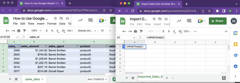
Step 3: Write the IMPORTRANGE Formula in Your Destination Sheet

Open the Google Sheet where you want the data to appear (your “Master Sales Dashboard”).
Select the cell where you want the imported data to begin (e.g., A1 on a new tab named Imported Sales Data).
Type the IMPORTRANGE formula using the URL and range string you just gathered.
Using our example:
```
=IMPORTRANGE("https://docs.google.com/spreadsheets/d/1abcde12345/edit#gid=0", "Data!A1:D100")
```
If using only the Spreadsheet ID:
```
=IMPORTRANGE("1abcde12345", "Data!A1:D100")
```
How to Use IMPORTRANGE to Pull Data from Other Sheets
Press Enter.

Step 4: Grant Permission (Crucial First Step!)

This is perhaps the most important part of How to Use IMPORTRANGE to Pull Data from Other Sheets, and a common point of confusion for new users.

When you first enter an IMPORTRANGE formula that links to a new spreadsheet, Google Sheets will display a #REF! error in the cell.
Hover over the cell with the #REF! error. You will see a prompt: “You need to connect these sheets. Allow access.”
Click the Allow access button.
How to Use IMPORTRANGE to Pull Data from Other Sheets

Important Note: You only need to grant permission once per unique source spreadsheet for your Google account. After that, any IMPORTRANGE formula linking to that same source sheet from any of your other sheets (within the same account) will work automatically. If you’re sharing the destination sheet, other users might need to grant access themselves if they are also editing the sheet, or if the source sheet’s sharing settings restrict access. Ensure the source sheet is shared appropriately (e.g., “Anyone with the link can view”) if multiple people need to see the imported data without individual permission grants.
Once access is granted, the data from your source sheet will populate the selected range in your destination sheet.

You have now successfully learned How to Use IMPORTRANGE to Pull Data from Other Sheets for a basic import!

Combining IMPORTRANGE with Other Powerful Functions

IMPORTRANGE is incredibly useful on its own, but its true power shines when combined with other Google Sheets functions. This allows you to not just pull data, but also process, filter, sort, and aggregate it directly as it’s imported. This is where your data analyst skills truly come into play, building sophisticated, dynamic reports.

Using IMPORTRANGE with QUERY for Filtering and Aggregating

The QUERY function is like a mini-database query language within Google Sheets. When combined with IMPORTRANGE, you can selectively import data based on criteria, summarize it, and much more.

Let’s continue our sales data example. Suppose you only want to see sales data for the “East” region and only for “Product A”, and you want to sum the sales amounts.

=QUERY(IMPORTRANGE("https://docs.google.com/spreadsheets/d/1abcde12345/edit#gid=0", "Data!A:D"), "SELECT Col1, Col2, Col3, Col4 WHERE Col2 = 'East' AND Col3 = 'Product A' ORDER BY Col1", 1)

Let’s break this down:

IMPORTRANGE("...", "Data!A:D"): This is our first argument for QUERY, providing the raw data table from the source sheet. Notice we’re importing entire columns A:D, as QUERY will do the filtering.
"SELECT Col1, Col2, Col3, Col4 WHERE Col2 = 'East' AND Col3 = 'Product A' ORDER BY Col1": This is the QUERY string.
- Col1, Col2, Col3, Col4: When IMPORTRANGE provides data to QUERY, it treats the imported columns as Col1, Col2, Col3, etc., regardless of their original column letters (A, B, C, D). So, Col2 refers to the Region column, Col3 to Product.
- WHERE Col2 = 'East' AND Col3 = 'Product A': Filters the data to only include rows where the region is ‘East’ AND the product is ‘Product A’.
- ORDER BY Col1: Sorts the results by the first column (Date).
1: This final argument in QUERY tells the function that the first row of the imported data is a header row, so it should be treated as such. If your imported data has no header row, you’d use 0.

To sum the sales for the “East” region and “Product A”:

=QUERY(IMPORTRANGE("https://docs.google.com/spreadsheets/d/1abcde12345/edit#gid=0", "Data!A:D"), "SELECT SUM(Col4) WHERE Col2 = 'East' AND Col3 = 'Product A'", 0)

Here, SUM(Col4) calculates the total of the fourth column (Sales Amount) after filtering. We use 0 for the header argument since we’re only returning a single sum, not a table with headers.

Using IMPORTRANGE with VLOOKUP/XLOOKUP for Cross-Sheet Lookups

While IMPORTRANGE pulls entire ranges, VLOOKUP or XLOOKUP (if available in your Sheets version) can retrieve specific pieces of information from a dynamically imported dataset.

Suppose you have a product ID in your current sheet and want to find its corresponding price from a “Product Catalog” sheet.

Source Sheet: “Product Catalog”

URL: https://docs.google.com/spreadsheets/d/1xyz789/edit#gid=0
Sheet Name: Catalog
Data Range: A:C (Columns: Product ID, Product Name, Price)

In your destination sheet, if you have a Product ID in cell A2, you can find its Price using:

=VLOOKUP(A2, IMPORTRANGE("https://docs.google.com/spreadsheets/d/1xyz789/edit#gid=0", "Catalog!A:C"), 3, FALSE)

A2: The lookup value (the Product ID you’re searching for).
IMPORTRANGE("...", "Catalog!A:C"): This is the table range for VLOOKUP, provided dynamically by IMPORTRANGE. VLOOKUP will search the first column (Product ID) of this imported data.
3: The column index from which to return a value (the 3rd column, which is Price).
FALSE: Ensures an exact match for the Product ID.

For XLOOKUP, which is more flexible:

=XLOOKUP(A2, IMPORTRANGE("https://docs.google.com/spreadsheets/d/1xyz789/edit#gid=0", "Catalog!A:A"), IMPORTRANGE("https://docs.google.com/spreadsheets/d/1xyz789/edit#gid=0", "Catalog!C:C"), "Not Found", FALSE)

How to Use IMPORTRANGE to Pull Data from Other Sheets

Here, we’re using IMPORTRANGE twice: once for the lookup range (Product IDs) and once for the return range (Prices). XLOOKUP is more versatile as the return range doesn’t have to be to the right of the lookup range.

Advanced IMPORTRANGE Techniques

Once you’re comfortable with the basics of How to Use IMPORTRANGE to Pull Data from Other Sheets and combining it with QUERY, you can explore more advanced scenarios.

Importing Multiple Sheets (Using `{}` Array Literals)

What if you have sales data spread across separate sheets for different months (e.g., “Jan Sales”, “Feb Sales”, “Mar Sales”) within the same source spreadsheet, and you want to combine them all into one continuous list? You can use IMPORTRANGE with array literals {}.

={
  IMPORTRANGE("https://docs.google.com/spreadsheets/d/1abcde12345/edit#gid=0", "Jan Sales!A:D");
  IMPORTRANGE("https://docs.google.com/spreadsheets/d/1abcde12345/edit#gid=0", "Feb Sales!A:D");
  IMPORTRANGE("https://docs.google.com/spreadsheets/d/1abcde12345/edit#gid=0", "Mar Sales!A:D")
}

The curly braces {} create an array.
The semicolon ; tells Google Sheets to stack the data vertically (append rows). If you wanted to combine them horizontally (append columns), you would use a comma ,.
Each IMPORTRANGE call brings in a separate dataset, and the array literal combines them.

Important Note: For this to work seamlessly, all imported ranges must have the same number of columns and the columns should represent the same data types in the same order. For instance, if “Jan Sales!A:D” has “Date, Region, Product, Sales” and “Feb Sales!A:E” has an extra column, this formula will return an error because the array structure would be inconsistent.

Dynamic Sheet IDs or Range Strings

Instead of hardcoding the spreadsheet_url or range_string directly into the IMPORTRANGE formula, you can refer to cells that contain these values. This makes your formulas more flexible and easier to update.

Let’s say cell A1 contains your spreadsheet_id and cell B1 contains your range_string.

=IMPORTRANGE(A1, B1)

This is incredibly useful for building dynamic dashboards where you might want to switch the source sheet or the range being imported by simply changing a value in a cell, rather than editing the formula itself.

Common Errors and How to Fix Them

Even experienced data analysts run into issues with IMPORTRANGE. Here are the most common errors and how to troubleshoot them:

1. `#REF!` Error: “You need to connect these sheets. Allow access.”

Cause: This is the most common first-time error. You haven’t granted permission for the destination sheet to access the source sheet.
Solution: Hover over the cell with the #REF! error and click the Allow access button when it appears. You only need to do this once per unique source spreadsheet per Google account.

2. `#REF!` Error: “Result was not expanded because it would overwrite data in…”

Cause: The IMPORTRANGE formula is trying to import data into cells that are already occupied.
Solution: Clear the cells to the right and below where your IMPORTRANGE formula starts. Ensure there’s enough empty space for all the data to be imported. If you’re importing a large range like A:D, ensure columns A, B, C, and D are entirely empty below your formula’s starting point.

3. `#ERROR!` Error: “Argument must be a range.” or “Invalid range string.”

Cause:
- Missing quotation marks around the spreadsheet_url or range_string.
- Incorrect sheet name or range format in the range_string (e.g., typos, extra spaces, incorrect cell references).
- Trying to import a range that doesn’t exist in the source sheet.
Solution:
- Double-check that both arguments are enclosed in double quotation marks.
- Verify the sheet name in your range_string exactly matches the sheet name in the source spreadsheet.
- Ensure the cell range (A1:D100 or A:D) is valid and refers to data that actually exists.
- Remember to use single quotes within double quotes for sheet names with spaces (e.g., " 'My Data'!A:B ").

4. `#N/A` Error (or blank cells when data should be there)

Cause:
- Permission issue (less common than #REF! for this).
- The IMPORTRANGE is successful, but there’s no data in the specified range on the source sheet.
- A QUERY function combined with IMPORTRANGE has very strict filter criteria that return no results.
- The spreadsheet_url or range_string refers to a non-existent sheet or incorrect range within the source document.
Solution:
- Manually open the source spreadsheet and confirm that the data exists in the exact sheet and range you specified in your IMPORTRANGE formula.
- If using QUERY, temporarily remove the WHERE clause to see if data imports, then re-add and refine your filters.

5. Slow Loading / Performance Issues

Cause:
- Too many IMPORTRANGE functions in one sheet, especially if they are pulling very large datasets.
- Nested IMPORTRANGE functions (e.g., IMPORTRANGE pulling from a sheet that itself uses IMPORTRANGE).
Solution:
- Consolidate IMPORTRANGE calls where possible. Instead of IMPORTRANGE five separate small ranges from the same sheet, use one IMPORTRANGE for a larger encompassing range and then use QUERY or other functions to filter that single import.
- Import only the necessary columns/rows. Avoid A:ZZZ if you only need A:C.
- Consider creating an “import tab” where you run all your raw IMPORTRANGEs, and then your main reports reference that tab, rather than having many IMPORTRANGEs directly in your report calculations. This creates a single point of data retrieval and often improves performance.

Best Practices for Using IMPORTRANGE

To truly master How to Use IMPORTRANGE to Pull Data from Other Sheets and ensure your spreadsheets are efficient, maintainable, and robust, follow these best practices:

Grant Access Proactively: Make it a habit to grant access immediately. If you’re building a sheet for others, guide them through this step.
Use Specific Ranges: Instead of A:ZZZ, use A:D or A1:D100 if you know your data bounds. This reduces the amount of data Google Sheets needs to process.
Name Your Sheets Clearly: Ensure sheet names in both source and destination are descriptive. This helps prevent typos in your range_string and makes formulas easier to read.
Centralize Source Data: Keep your “master” data in dedicated, well-organized source sheets. This simplifies maintenance and debugging.
Dedicated Import Tabs: For complex dashboards or reports, create a separate tab (e.g., _RawData_) solely for your IMPORTRANGE formulas. Your other tabs can then reference this _RawData_ tab. This improves organization, performance, and makes troubleshooting much easier.
Avoid Nesting IMPORTRANGE (if possible): While technically feasible, pulling data from a sheet that itself imports data can create a chain of dependencies that are slow and harder to manage. Try to link directly to the primary source whenever possible.
Share Responsibly: Ensure the source sheet has appropriate sharing permissions (“Viewer” access for “Anyone with the link” is common for public data, or specific user access for private data) so that anyone who needs to see the imported data can.

Conclusion

By now, you should have a solid understanding of How to Use IMPORTRANGE to Pull Data from Other Sheets. This isn’t just a simple function; it’s a gateway to building highly dynamic, interconnected, and automated spreadsheet systems. From basic data consolidation to complex filtering and aggregation with QUERY, IMPORTRANGE empowers you to centralize information, reduce errors, and save countless hours previously spent on manual data transfer.

Embrace IMPORTRANGE as a core tool in your Google Sheets toolkit. The ability to pull live data from disparate sources into a single, cohesive view will undoubtedly elevate your productivity and the accuracy of your reports, making you a true spreadsheet wizard in any office or academic setting. Start experimenting with these techniques today, and watch your data management challenges fade away!

Frequently Asked Questions (FAQ)

Q1: Can IMPORTRANGE pull data from an Excel file or other non-Google Sheets files?

A1: No, IMPORTRANGE is specifically designed for pulling data between Google Sheets files only. For importing data from Excel, you would first need to upload the Excel file to Google Drive and convert it to a Google Sheet, or use a third-party add-on if direct connection is required.

Q2: What happens if the source spreadsheet is deleted or moved?

A2: If the source spreadsheet’s URL changes (e.g., it’s moved to a different folder and a new sharing link is generated) or if it’s deleted entirely, your IMPORTRANGE formula will return a #REF! error, indicating that the source could not be found. You would need to update the spreadsheet_url in your formula to the correct new URL or restore the sheet.

Q3: Does IMPORTRANGE automatically update data, or do I need to refresh it?

A3: IMPORTRANGE updates automatically, typically within a few seconds to a few minutes, when changes occur in the source sheet. Google Sheets manages this refresh in the background. For very large datasets or complex sheets, there might be a slight delay, but it’s generally considered real-time for most practical purposes.

Q4: Can I use IMPORTRANGE if the source sheet is private and not shared with me?

A4: No. You must have at least “Viewer” access to the source spreadsheet for IMPORTRANGE to work. If you don’t have access, you’ll encounter a permission error or a #REF! error after attempting to grant access. The owner of the source sheet must grant you explicit view permissions.

Q5: Can I import only specific columns, not necessarily a contiguous range?

A5: Directly with IMPORTRANGE, you can only import a contiguous rectangular range (e.g., A:C). However, you can achieve the effect of importing specific, non-contiguous columns by wrapping IMPORTRANGE within a QUERY function. For example, QUERY(IMPORTRANGE("url", "Sheet1!A:Z"), "SELECT Col1, Col5, Col10") would import only the 1st, 5th, and 10th columns from your imported data.

See more: How to Use IMPORTRANGE to Pull Data from Other Sheets.

Discover: AskByteWise.