Ever found yourself lost in a sprawling Excel spreadsheet, frantically scrolling up and down, left and right, trying to remember what that number in column AG actually referred to? We’ve all been there. It’s a common productivity killer, a frustrating drain on your focus and time management that can turn a simple data analysis task into a daunting challenge. This constant loss of context can derail your workflow, making it harder to maintain data accuracy and achieve your goal setting targets.
But what if you could anchor your essential headers – those crucial row and column labels – in place, no matter how far you scroll? Imagine the clarity, the peace of mind, the sheer efficiency! That’s exactly what we’re going to achieve today. Welcome to the definitive guide on how to Freeze Panes in Excel to lock rows and columns, a simple yet powerful feature that will fundamentally transform the way you interact with large datasets. It’s not just a trick; it’s a foundational skill for anyone looking to master Excel and elevate their professional productivity.
The Unseen Productivity Drain: Why Endless Scrolling Sabotages Your Workflow
In today’s data-driven world, Excel isn’t just a tool; it’s often the backbone of our daily operations. From tracking project budgets and managing customer lists to analyzing scientific data or preparing for crucial presentations, spreadsheets are ubiquitous. But with great power comes great complexity, and nothing saps your energy like a gargantuan sheet where your headers vanish into the digital ether.
Think about a student analyzing survey results for a thesis, needing to correlate responses across dozens of questions. Or a project manager tracking tasks, budgets, and team assignments, with each row representing a project deliverable and each column detailing its status, owner, and deadline. Now, imagine trying to update a task far down the list, and having to scroll all the way back up to remind yourself which column holds the “Due Date” and which one tracks “Completion Percentage.” Frustrating, isn’t it?
This constant mental gymnastics of “where was that column?” or “what does this row even represent?” isn’t just annoying; it has tangible consequences:
- Increased Errors: When you lose context, the likelihood of entering data into the wrong cell or misinterpreting information skyrockets.
- Wasted Time: Each scroll and re-orientation costs precious seconds, which quickly accumulate into minutes, then hours, especially in collaborative environments where multiple people are interacting with the same data.
- Cognitive Overload: Your brain expends unnecessary energy trying to keep track of information that should be readily available, leaving less capacity for actual analysis and decision-making.
- Reduced Focus****: The constant interruption breaks your concentration, making it harder to get into a state of deep work.
It’s clear: mastering your digital workspace is key to mastering your tasks. And that’s where knowing how to Freeze Panes in Excel to lock rows and columns comes in as an indispensable ally.
What Exactly Are Freeze Panes? Your Anchor in a Sea of Data
At its core, Freeze Panes is an Excel feature designed to keep specific rows and/or columns visible as you scroll through the rest of your worksheet. Think of it like pinning important notes to the top or side of a large canvas. No matter where you move your viewpoint on the canvas, those pinned notes remain fixed, providing constant reference.
For a large Excel sheet, this means your column headers (like “Employee Name,” “Sales Region,” “Project Status”) and/or your row labels (like “January,” “Region North,” “Product XYZ”) will always be on display. This makes navigating vast amounts of information not just easier, but intuitively clear. It transforms a potentially overwhelming spreadsheet into an organized, manageable tool for data analysis and decision-making.
It’s a small change with a massive impact on your daily efficiency and productivity. Whether you’re a student dissecting a complex dataset, a financial analyst sifting through quarterly reports, or a small business owner managing inventory, understanding how to Freeze Panes in Excel to lock rows and columns is a fundamental step towards reclaiming your time management and enhancing your overall workflow.
Unlock Clarity: The Core Benefits of Freezing Panes
The power of learning how to Freeze Panes in Excel to lock rows and columns extends far beyond simply seeing your headers. It’s about fundamentally changing your interaction with data, making it more intuitive, less error-prone, and ultimately, more productive.
Here are the key benefits you’ll experience:
- Uninterrupted Context and Focus**: This is the most immediate and profound benefit. You’ll never again have to scroll back up or left to identify what data point you’re looking at. Your essential labels are always visible, allowing you to maintain a steady focus** on the actual data and analysis.
- Enhanced Data Accuracy**: With constant visibility of your headers, the chances of misinterpreting data or entering it into the wrong cell are drastically reduced. This is crucial for maintaining the integrity of your spreadsheets, especially in collaborative** projects where multiple users might be inputting information.
- Improved Workflow** and Efficiency**: Navigating large datasets becomes seamless. You spend less time scrolling and searching, and more time actually working with the data. This streamlines your workflow, saving valuable minutes that add up over a day or week.
- Simplified Collaboration**: When sharing spreadsheets with colleagues, frozen panes provide a clear and consistent viewing experience for everyone. This reduces confusion and helps ensure that all team members are on the same page, fostering better collaboration** and shared understanding.
- Professional Presentation: For anyone presenting data, frozen panes ensure that key identifiers are always visible, even as you navigate through the sheet. This makes your presentations clearer, more professional, and easier for your audience to follow, enhancing your authoritativeness.
- Reduced Cognitive Load: By removing the need to constantly re-orient yourself, Freeze Panes frees up your mental energy. This allows you to dedicate more brainpower to critical thinking, problem-solving, and achieving your goal setting objectives, rather than remembering column names.
- Empowering Time Management**: By making your Excel experience more efficient, Freeze Panes directly contributes to better time management**. You get tasks done faster, freeing up time for more strategic work or personal pursuits.
“The true measure of efficiency is not how much you do, but how much you get done without wasting precious mental energy on avoidable friction.” – AskByteWise.com Principle
How to Freeze Panes in Excel: A Step-by-Step Guide
Learning how to Freeze Panes in Excel to lock rows and columns is surprisingly straightforward. Excel offers three main options, catering to different needs. We’ll walk through each method, ensuring you’re equipped to handle any spreadsheet scenario.
Before You Start: It’s a good practice to save your work before making significant changes, though freezing panes is generally a safe operation. Also, ensure you have a basic understanding of your spreadsheet’s layout – which rows are headers, and which columns are key identifiers.
1. Freezing the Top Row (For Column Headers)
This is the most common use case, perfect for when your column headers are in the first row, and you need them to remain visible as you scroll down.
- Select Any Cell: You don’t need to select the entire row. Just click on any cell in your worksheet.
- Navigate to the View Tab: In the Excel ribbon at the top of your screen, click on the “View” tab.
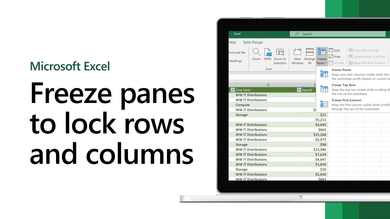
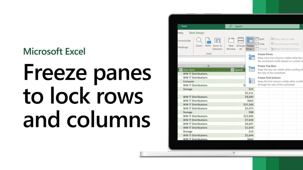
- Locate Freeze Panes: In the “Window” group (usually towards the middle or right of the View tab), click the “Freeze Panes” dropdown button.
- Choose “Freeze Top Row”: From the options that appear, select “Freeze Top Row.”
That’s it! A thin line will appear just below the first row, indicating that it’s now locked. Scroll down, and you’ll see your top row stays put.
2. Freezing the First Column (For Row Labels)
Useful when your primary row labels (like names, dates, or product IDs) are in the first column, and you need them to stay visible as you scroll horizontally to the right.
- Select Any Cell: Again, any cell in the worksheet will do.
- Navigate to the View Tab: Click on the “View” tab in the Excel ribbon.
- Locate Freeze Panes: In the “Window” group, click the “Freeze Panes” dropdown button.
- Choose “Freeze First Column”: Select “Freeze First Column” from the options.
A thin line will appear to the right of the first column, signifying it’s now frozen. Scroll right, and your first column will remain in view.
3. Freezing Both Rows and Columns (Specific Area)
This is the most versatile option and often the most powerful for complex datasets. It allows you to freeze multiple rows at the top and multiple columns on the left simultaneously.
- Identify Your Freeze Point: This is the crucial step. You need to select the cell immediately below the rows you want to freeze and immediately to the right of the columns you want to freeze.
- Example: If you want to freeze the first three rows (rows 1, 2, 3) and the first two columns (columns A, B), you would select cell C4. Cell C4 is below row 3 and to the right of column B.
- Tip: Think of the selected cell as the “corner” of your unfrozen area. Everything above and to the left of it will be frozen.
- Navigate to the View Tab: Click the “View” tab.
- Locate Freeze Panes: In the “Window” group, click the “Freeze Panes” dropdown button.
- Choose “Freeze Panes”: This time, select the top option: “Freeze Panes” (not “Freeze Top Row” or “Freeze First Column”).
Now, a horizontal line will appear below your frozen rows, and a vertical line to the right of your frozen columns. Both sets of headers will remain visible as you navigate your spreadsheet.
Unfreezing Panes: Reclaim Your Canvas
If you need to change your frozen area or simply want to revert to a fully scrollable sheet, unfreezing is just as easy:
- Select Any Cell: It doesn’t matter which one.
- Navigate to the View Tab: Click the “View” tab.
- Locate Freeze Panes: In the “Window” group, click the “Freeze Panes” dropdown.
- Choose “Unfreeze Panes”: Select “Unfreeze Panes” from the options.
All frozen areas will disappear, and your sheet will be fully scrollable again. Remember, you must unfreeze panes before you can refreeze them in a new location.
Beyond the Basics: Advanced Tips for Maximizing Your Frozen Views
Simply knowing how to Freeze Panes in Excel to lock rows and columns is a great start, but understanding some nuances can elevate your experience and truly supercharge your workflow.
Consider Multi-Row Headers
Many professional spreadsheets aren’t content with just one row of headers. You might have a main header row, followed by sub-category headers. For instance:
| Month | Region | Quarter 1 Sales | Quarter 1 Profit | Quarter 2 Sales | Quarter 2 Profit |
|---|---|---|---|---|---|
| Product A | Product B | Product A | Product B |
In such cases, you’d want to freeze both rows 1 and 2. To do this, you would select cell A3 (or B3, C3, etc. – any cell in row 3). Then go to View > Freeze Panes > Freeze Panes. This ensures both your main and sub-headers remain visible, maintaining full context.
Freezing Multiple Columns (and Rows)
While the “Freeze First Column” option only freezes, well, the first column, the “Freeze Panes” command allows you to freeze any number of leading columns. If your important identifiers stretch across columns A, B, and C, you would select a cell in column D (e.g., D1 to freeze just columns A-C, or D2 if you also want to freeze the top row). This flexibility is vital for wide datasets where multiple columns contain essential identifiers.
Zooming and Freeze Panes
Be aware that when you zoom in or out of your worksheet, the size of your frozen panes will scale accordingly. This is usually helpful, as it maintains the visual integrity. However, if you find your frozen headers becoming too large or too small, adjust your zoom level (in the View tab) or simply unfreeze and refreeze if necessary.
Using Tables and Freeze Panes Together
Excel Tables (Insert > Table) offer their own form of “sticky headers.” When you convert a range into an Excel Table, the header row automatically becomes visible in the worksheet frame as you scroll down, even without using Freeze Panes. However, Table headers don’t stick when scrolling horizontally. For comprehensive locking (both rows and columns), you’ll still need to use Freeze Panes in conjunction with Tables, or simply use Freeze Panes on its own if you don’t need other Table functionalities. This combination can be particularly powerful for advanced data analysis and organization.
Integrating Freeze Panes into Your Daily Workflow: Smart Habits for Smarter Spreadsheets
Knowing how to Freeze Panes in Excel to lock rows and columns is the first step; making it a habit is where the real productivity gains lie. Here are some smart ways to seamlessly integrate this feature into your daily routine.
Proactive Freezing
Don’t wait until you’re lost in a sea of data to freeze panes. Make it one of the first things you do when opening a large or complex spreadsheet. Treat it like setting up your workspace: clear your desk, open your necessary tools, and then freeze your panes. This proactive approach will save you countless moments of frustration later on, improving your overall time management.
Leverage for Collaboration
When preparing spreadsheets for collaboration or sharing with others, always consider if freezing panes would improve their experience. By setting up the most logical frozen view (e.g., freezing crucial ID columns and header rows), you’re making the document more accessible and user-friendly for your colleagues. This demonstrates your expertise and fosters smoother teamwork.
Tailor to Your Task
The best freeze pane setup isn’t always the same. If you’re focused on data entry, you might want to freeze more columns to keep key identifiers visible. If you’re performing data analysis and comparing figures across many rows, freezing the top row might be sufficient. Adapt your freeze pane strategy to the specific task at hand to maximize efficiency.
Teach Others
One of the best ways to solidify your own knowledge and enhance your team’s overall workflow is to share what you’ve learned. Teach your colleagues, fellow students, or team members how to Freeze Panes in Excel to lock rows and columns. This not only spreads efficiency but also positions you as a valuable resource and expert within your group.
Regular Review and Adjustment
As your spreadsheet evolves, so might your needs for frozen panes. If new columns or rows become critical identifiers, or if the layout changes, take a moment to unfreeze and re-freeze your panes. A quick adjustment can prevent future frustration and keep your focus sharp. It’s part of a continuous improvement mindset for your digital workspace.
Conclusion: Anchor Your Data, Elevate Your Efficiency
The journey to mastering Excel, and indeed any powerful software, is paved with understanding these seemingly small, yet profoundly impactful features. Learning how to Freeze Panes in Excel to lock rows and columns is more than just a technical skill; it’s a strategic move towards better time management, enhanced focus, and superior workflow.
No longer will you be adrift in endless scrolling, desperately seeking context. With your crucial headers and labels firmly anchored, you’ll navigate your datasets with newfound clarity and confidence. This simple trick reduces cognitive load, minimizes errors, and empowers you to dedicate your mental energy to what truly matters: understanding your data, making informed decisions, and achieving your goal setting objectives.
At AskByteWise.com, our mission is “Making Complex Tech Simple,” and few features exemplify this better than Freeze Panes. It’s an accessible tool that yields immediate, tangible benefits for students, professionals, and anyone who interacts with data. Embrace this powerful feature today, and watch as your efficiency soars, turning spreadsheet frustration into productive mastery. Go forth, freeze those panes, and unlock a more focused, effective you!
Frequently Asked Questions (FAQ)
Q1: Can I freeze multiple non-contiguous rows or columns?
No, Excel’s Freeze Panes feature only allows you to freeze rows at the top of your worksheet and columns at the left of your worksheet. You cannot freeze a row in the middle of your sheet while leaving the rows above it unfrozen, or similarly for columns. If you need to focus on specific, non-contiguous data, consider using Excel’s Filter feature, hiding rows/columns, or creating a separate summary table.
Q2: What’s the difference between “Freeze Panes,” “Freeze Top Row,” and “Freeze First Column”?
- Freeze Top Row: Locks only the very first row (Row 1) of your sheet. Useful when your primary column headers are in Row 1.
- Freeze First Column: Locks only the very first column (Column A) of your sheet. Useful when your primary row labels are in Column A.
- Freeze Panes (the general option): This is the most versatile. You select a cell, and everything above that cell’s row and to the left of that cell’s column will be frozen. This allows you to freeze multiple top rows and multiple left-hand columns simultaneously, giving you precise control over your visible headers.
Q3: Why can’t I select “Freeze Panes”? It’s grayed out.
This usually happens if you are in “Page Break Preview” or “Page Layout” view. Freeze Panes only works in “Normal” view. To switch back to Normal view, go to the View tab on the Excel ribbon and click “Normal” in the “Workbook Views” group. If it’s still grayed out, ensure you don’t have multiple Excel windows open that might be interfering, or try restarting Excel.
Q4: Does Freeze Panes affect printing?
No, Freeze Panes only affects how you view the worksheet on your screen; it does not impact how your spreadsheet prints. If you want specific rows or columns to repeat on every printed page, you need to use the “Print Titles” feature (found in the Page Layout tab > Print Titles).
Q5: Can I freeze panes on a specific table within a larger sheet?
Freeze Panes applies to the entire worksheet, not just a specific table range within it. If you convert your data into an Excel Table (Insert > Table), the table’s header row will automatically become “sticky” as you scroll vertically within the table, even without using Freeze Panes. However, this won’t freeze columns or other rows, so for comprehensive locking, you’d still use the main Freeze Panes feature based on the overall worksheet layout.
See more: How to Freeze Panes in Excel to Lock Rows and Columns.
Discover: AskByteWise.