Master Your Data: How to Freeze Panes in Excel to Lock Rows and Columns

Ever felt like you’re navigating a vast ocean of numbers in Excel, constantly scrolling, losing your bearings, and frantically trying to remember which column header belonged to which set of data? It’s a common struggle, whether you’re a student crunching research data, a professional managing a complex project budget, or an entrepreneur tracking sales figures. This constant back-and-forth isn’t just annoying; it’s a massive drain on your focus, a significant hit to your time management, and a silent killer of your overall productivity.

But what if there was a simple, elegant solution to this data dilemma? A way to keep those crucial headers and labels always in sight, no matter how far down or across your spreadsheet you venture? Welcome to the world of Freezing Panes in Excel to Lock Rows and Columns. This isn’t just a basic Excel trick; it’s a powerful feature that can revolutionize your workflow, enhance your data analysis, and bring an unprecedented level of clarity to your complex spreadsheets. As a content strategist dedicated to making complex tech simple, I’m here to guide you through mastering this essential tool. Let’s unlock a new level of efficiency together.

The Hidden Power of Frozen Panes: Why Your Workflow Needs It

Imagine you’re reviewing a financial report spanning hundreds of rows and dozens of columns. Your critical headers – ‘Quarter 1 Sales’, ‘Marketing Spend’, ‘Net Profit’ – disappear the moment you scroll down. Your key identifiers – ‘Product ID’, ‘Customer Name’ – vanish as you scroll right. This isn’t just an inconvenience; it’s a cognitive overload. You’re constantly switching contexts, trying to remember what each number represents, leading to errors, frustration, and wasted time.

This is precisely where freezing panes becomes your digital anchor, a steadfast companion in the turbulent seas of your data. It’s a fundamental feature that directly impacts your efficiency and accuracy, turning a chaotic experience into a streamlined one.

Let’s break down the transformative benefits:

Enhanced Focus and Clarity: When your essential headers and labels remain visible, your brain doesn’t have to work overtime recalling context. This significantly reduces cognitive load, allowing you to focus directly on the data and its implications. No more guessing, no more second-guessing.
Improved Data Analysis: Analyzing large datasets becomes a breeze. You can easily compare values across different categories or periods without losing sight of what you’re comparing. This leads to deeper insights and more informed decision-making, which is crucial for effective goal setting.
Seamless Collaboration: Sharing spreadsheets with frozen panes makes them instantly more understandable for collaborators. They don’t have to spend time figuring out the layout or asking for clarification. This fosters smoother collaboration and reduces communication overhead.
Significant Time Management Savings: The time saved from not having to scroll back and forth, or re-identify columns, accumulates rapidly. This efficiency gain translates into hours freed up for more critical tasks, directly impacting your time management.
Reduced Errors and Increased Trustworthiness: When context is always present, the likelihood of entering data in the wrong column or misinterpreting a value decreases dramatically. This boosts the trustworthiness of your data and, by extension, your reports and analyses.

“Productivity is never an accident. It is always the result of a commitment to excellence, intelligent planning, and focused effort.” – Paul J. Meyer

Freezing panes isn’t just about locking cells; it’s about locking in your concentration, securing your context, and elevating your overall workflow to a professional standard. It’s a testament to the idea that small changes in your technical habits can lead to monumental shifts in your productive output.

Understanding Your Options: The Different Ways to Freeze Panes

Excel, in its wisdom, understands that different data structures require different freezing strategies. You’re not always looking to lock everything; sometimes, just the top row is enough, or perhaps only the first column. This flexibility ensures that the feature adapts to your specific needs, rather than forcing your data into a rigid structure.

There are three primary ways to utilize the Freeze Panes feature, each designed for a particular scenario:

Freeze Top Row: This is ideal when your dataset has a header row (often Row 1) that describes the content of each column. Think of a sales report where the first row contains ‘Product Name’, ‘Units Sold’, ‘Revenue’, etc.
Freeze First Column: Perfect for datasets where the leftmost column acts as a primary identifier for each row. Examples include employee lists with ‘Employee ID’ in the first column, or research data with ‘Participant Code’.
Freeze Panes (Specific Rows and Columns): This is the most versatile option. It allows you to lock both a set of top rows and a set of left-most columns simultaneously. This is your go-to when you have multiple header rows (e.g., a main header and a sub-header row) or when your left-side identifiers also span multiple columns. This is where a little upfront planning makes a huge difference in your data management.

Let’s dive into the practical steps for each of these options.

Your Step-by-Step Guide: How to Freeze Panes in Excel

Ready to banish spreadsheet confusion for good? Follow these simple, clear instructions. Remember, the key is to understand what you want to see fixed and how Excel interprets your selection.

Before you begin, ensure you have your Excel workbook open and the sheet you want to modify is active.

Option 1: Locking Just the Top Row

This is the simplest and most common use case. It ensures that the very first row of your spreadsheet (Row 1) remains visible as you scroll down.

Navigate to the View Tab: In your Excel ribbon, locate and click on the “View” tab. This tab is where all your display-related tools live.
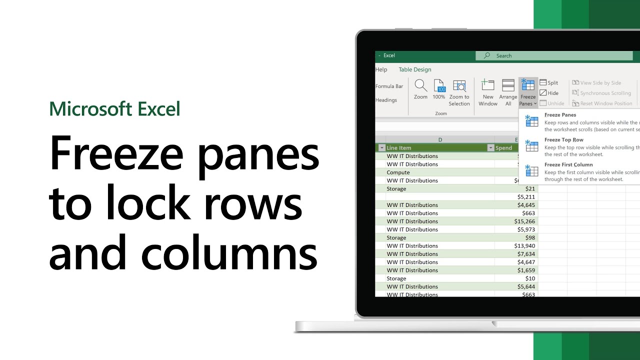
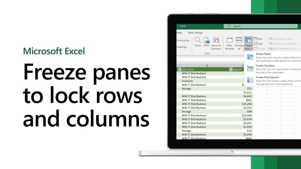
Locate Freeze Panes: Within the “View” tab, look for the “Window” group. Here, you’ll find the “Freeze Panes” dropdown button. Click it.
Select “Freeze Top Row”: From the dropdown menu, choose the option “Freeze Top Row”.

That’s it! You’ll notice a subtle, thin line appearing just below Row 1. Now, try scrolling down your spreadsheet. Row 1 will stay put, always in view. This simple action significantly boosts your focus when dealing with extensive lists.

Pro Tip: This option is perfect for any table where your column headers are neatly contained in the first row. It’s a quick win for instant clarity.

Option 2: Locking Just the First Column

Similar to freezing the top row, this option is designed to keep the leftmost column (Column A) visible as you scroll horizontally across your data.

Navigate to the View Tab: Click on the “View” tab in the Excel ribbon.
Locate Freeze Panes: In the “Window” group, click the “Freeze Panes” dropdown button.
Select “Freeze First Column”: From the dropdown menu, select the option “Freeze First Column”.

You’ll now see a thin line appearing to the right of Column A. Scroll right, and Column A will remain visible, making it much easier to track individual records or categories. This feature is particularly useful for improving your workflow on wide datasets.

Pro Tip: Use this when the first column contains unique identifiers like product codes, customer names, or project IDs, and you frequently need to scroll right to see associated data.

Option 3: Freezing Both Rows and Columns (The “Sweet Spot”)

This is where the magic truly happens. When you need to lock a specific number of rows and a specific number of columns, the standard “Freeze Panes” option gives you complete control. This is the most powerful method for complex data analysis.

The key to this method lies in understanding Excel’s logic: Excel freezes everything above and to the left of your currently selected active cell.

Identify Your Freeze Point: Determine the exact intersection where you want your frozen area to end. For example, if you want to freeze the first three rows (Rows 1-3) and the first two columns (Columns A-B), your intersection point is just below Row 3 and just to the right of Column B.
Select the “Active Cell”: Click on the cell that is one row below your last desired frozen row, AND one column to the right of your last desired frozen column.
- Example: To freeze Rows 1-3 and Columns A-B, you would click on Cell C4. (C is one column right of B, 4 is one row below 3).
- Example: To freeze Row 1 and Column A, you would click on Cell B2.
- Example: To freeze Rows 1-5 and Column A, you would click on Cell B6.
Navigate to the View Tab: Go to the “View” tab.
Select “Freeze Panes”: In the “Window” group, click the “Freeze Panes” dropdown button, and this time, select the first option: “Freeze Panes”.

Immediately, you’ll see a horizontal line and a vertical line appear, marking your frozen regions. Scroll around, and you’ll find both your selected top rows and left columns locked firmly in place. This level of control is paramount for advanced data management and collaboration.

Pro Tip: This method requires a bit more thought about your data layout, but once you master selecting the correct active cell, it becomes incredibly intuitive and powerful.

Unfreezing Panes: Reclaiming Your Full View

What if you’ve frozen panes and now want to go back to the normal, scrolling view? It’s just as simple to undo.

Navigate to the View Tab: Click on the “View” tab.
Locate Freeze Panes: In the “Window” group, click the “Freeze Panes” dropdown.
Select “Unfreeze Panes”: The option will now be “Unfreeze Panes” (it replaces “Freeze Panes” when panes are already frozen). Click it.

All frozen panes will disappear, and your spreadsheet will revert to its standard scrolling behavior.

Integrating Freeze Panes for Peak Productivity and Smart Collaboration

Mastering “How to Freeze Panes in Excel to Lock Rows and Columns” is more than just learning a feature; it’s about integrating a smart practice into your daily routine that significantly uplifts your productivity and the quality of your collaboration. This simple tool, when applied thoughtfully, can be a cornerstone of effective time management and data clarity.

Let’s explore how to make this a habit and why it matters in various scenarios:

Real-World Scenarios Where Freeze Panes Shines:

Financial Analysts and Accountants: Imagine working on an annual budget, where the first few rows contain department names, and the first column lists months. Freezing both allows you to easily input and compare figures across departments and time periods without losing context. This ensures accurate financial reporting and helps in goal setting.
Project Managers: Tracking a large project often involves a spreadsheet with task IDs, owner names, and deadlines in the initial columns, and weekly progress updates stretching across many columns. Freezing the initial columns keeps the task details visible as you scroll to update progress for upcoming weeks. This streamlines workflow and enhances project collaboration.
Students and Researchers: When compiling research data – perhaps survey results or experimental observations – you might have participant IDs or variables in the first column, and different metrics or questions in the top row. Freezing these ensures you’re always associating the right data with the right participant and metric, maintaining data integrity and easing analysis for your academic pursuits.
Sales and Marketing Teams: Analyzing customer databases or lead lists where the first column has customer names/IDs and the top row has various demographic or interaction metrics. Freezing panes helps in segmenting and understanding customer behavior, directly contributing to marketing goal setting.

Tips for Optimal Use and Integration:

Make it a First Step: Whenever you open a large, complex spreadsheet that you’ll be interacting with heavily, make freezing panes one of your very first actions. It’s a small investment of time that pays huge dividends in saved frustration.
Teach Your Team: If you’re working in a shared environment, encourage your colleagues to use frozen panes. A quick 30-second demonstration can drastically improve team-wide collaboration and data efficiency. When everyone is on the same page, the collective workflow improves.
Combine with Other Excel Features: Frozen panes work beautifully with other tools. For instance, you can use frozen panes in conjunction with data filtering to analyze specific subsets of data while still keeping your headers visible. Or, combine with sorting to organize your data and then use frozen panes to navigate the organized view with ease.
Regular Review: As your data evolves, your freeze pane needs might change. Periodically review if your current frozen areas are still optimal. Don’t hesitate to unfreeze panes and re-apply them to better suit your current analytical task.

“The secret of getting ahead is getting started. The secret of getting started is breaking your complex overwhelming tasks into small manageable tasks, and then starting on the first one.” – Mark Twain

This powerful yet simple feature embodies AskByteWise.com’s mission: “Making Complex Tech Simple.” It’s about leveraging the tools at your disposal to create a more efficient, less overwhelming digital environment. By integrating freezing panes into your standard Excel practice, you’re not just locking rows and columns; you’re locking in greater focus, superior time management, and a smoother workflow for every task.

Common Pitfalls and How to Avoid Them

Even with a tool as straightforward as Freeze Panes, a few common missteps can lead to unexpected results. Being aware of these can save you time and frustration.

Forgetting to Unfreeze Panes: You might set up frozen panes for one task, then move to another part of the sheet or another sheet entirely, forgetting that panes are still frozen. This can make navigation seem “stuck.” Always remember the “Unfreeze Panes” option when you no longer need the lock.
Selecting the Wrong Cell Before Freezing (for Option 3): This is the most frequent mistake. If you want to freeze Rows 1-5 and Columns A-C, and you accidentally select cell D5 instead of D6, you’ll find that only Rows 1-4 are frozen. Always double-check that your active cell is below your last desired frozen row and to the right of your last desired frozen column. A moment of precision here saves much more time later.
Attempting to Freeze Non-Contiguous Rows/Columns: The “Freeze Panes” feature is designed to lock contiguous rows from the top and contiguous columns from the left. You cannot, for example, freeze Row 1 and Row 5 simultaneously while leaving Rows 2-4 unfrozen using this method. If you need a more flexible view, consider using Excel’s “Split Window” feature, which allows for multiple independent scrolling regions (though it doesn’t “lock” them in the same way).
Confusing Freeze Panes with Locking Cells for Editing: Freezing panes is purely a viewing aid; it doesn’t prevent data entry or modification. If your goal is to prevent others from changing certain cells, you need to use Excel’s “Protect Sheet” feature, which is a different function entirely.

Conclusion: Unlock Your Spreadsheet’s Full Potential

In a world teeming with data, the ability to navigate and understand your information efficiently is no longer a luxury—it’s a necessity. The simple, yet profoundly effective, technique of “How to Freeze Panes in Excel to Lock Rows and Columns” stands as a testament to AskByteWise.com’s mission: “Making Complex Tech Simple.”

By implementing this feature, you’re not just learning a trick; you’re adopting a smarter workflow, reclaiming valuable time management, and cultivating a heightened sense of focus in your daily tasks. Whether you’re a student striving for academic excellence, a professional aiming to streamline reports, or anyone wrestling with extensive datasets, freezing panes empowers you to work with greater clarity, confidence, and precision.

Stop the endless scrolling and the frustrating loss of context. Take control of your data, enhance your collaboration, and elevate your productivity starting today. Open your next large Excel sheet and apply this invaluable skill. You’ll wonder how you ever managed without it. Embrace this elegant solution and transform your interaction with spreadsheets forever!

Frequently Asked Questions (FAQ)

Q1: Can I freeze multiple non-adjacent rows or columns?

No, the standard “Freeze Panes” feature in Excel is designed to lock contiguous rows from the top and contiguous columns from the left. You cannot freeze, for example, Row 1 and Row 5 without also freezing Rows 2, 3, and 4. If you need to view non-adjacent sections simultaneously, consider using the “Split Window” feature (found next to “Freeze Panes” on the View tab), which divides your worksheet into separate scrollable panes. However, these split panes don’t “lock” in the same way that frozen panes do.

Q2: Why is my “Freeze Panes” option grayed out?

If the “Freeze Panes” option is unavailable (grayed out), it’s usually for one of these reasons:

You’re in Cell Edit Mode: You might be actively editing a cell’s content. Press Enter or Esc to exit edit mode.
Workbook is Protected: The worksheet or workbook might be protected. You’ll need to unprotect it first (Review tab > Unprotect Sheet/Workbook).
Shared Workbook: In some older versions of Excel, “Freeze Panes” might be limited in a shared workbook.
Object Selected: If you have a chart, picture, or another object selected, deselect it first.

Q3: Does freezing panes affect printing?

No, freezing panes is purely a viewing feature within Excel and has no effect on how your spreadsheet will print. When you print, Excel will print the entire sheet based on your print area and page setup settings, regardless of whether panes were frozen or not.

Q4: What’s the difference between “Freeze Panes” and “Split Window”?

Freeze Panes: Locks specific rows (from the top) and/or columns (from the left) so they are always visible while you scroll the rest of the sheet. The frozen area remains static. It’s great for keeping headers/labels in sight for data analysis and focus.
Split Window: Divides your worksheet into two or four separate panes, each with its own scroll bars. You can scroll each pane independently. This is useful for viewing different, non-adjacent parts of a very large sheet at the same time, but it doesn’t “lock” them in the same fixed way as freezing.

Q5: Will frozen panes save with my Excel workbook?

Yes, absolutely! When you save your Excel workbook after freezing panes, the frozen pane settings are saved along with the file. The next time you (or anyone else) opens that workbook, the panes will be frozen exactly as you left them, ensuring consistent workflow and collaboration for anyone interacting with your data.

See more: How to Freeze Panes in Excel to Lock Rows and Columns.

Discover: AskByteWise.