Your First Spreadsheet: The Ultimate Guide to Google Sheets for Beginners

Are you tired of manually tracking data, performing repetitive calculations, or struggling to make sense of endless rows and columns? Do you dream of a world where your data works for you, not the other way around? Welcome to The Ultimate Guide to Google Sheets for Beginners! As Noah Evans, lead content strategist at AskByteWise.com, my mission is to demystify complex tech, and today, we’re diving deep into the world of Google Sheets. This powerful, cloud-based spreadsheet application is a game-changer for office professionals and students alike, offering robust tools for organizing, analyzing, and visualizing data. Whether you’re managing budgets, tracking project progress, or analyzing sales figures, this comprehensive guide will equip you with the foundational skills to master Google Sheets and transform the way you work with data. Let’s make complex tech simple, together!

Getting Started with Google Sheets

Before we dive into formulas and functions, let’s understand what Google Sheets is and why it’s become an indispensable tool for millions.

What is Google Sheets?

Think of Google Sheets as your smart, super-organized digital ledger. Instead of paper, you have a vast grid of cells where you can enter text, numbers, dates, and even complex formulas. It’s part of Google’s free, web-based office suite, similar to how Google Docs is a word processor and Google Slides is for presentations. The beauty of Google Sheets lies in its accessibility and collaborative power.

Why Use Google Sheets?

Cloud-Based & Accessible: No software installation needed! Access your spreadsheets from any device, anywhere, with just a web browser. Your data is saved automatically to Google Drive.
Collaborative Powerhouse: Share your spreadsheets with colleagues or classmates and work on them simultaneously. See changes in real-time, making teamwork incredibly efficient.
Free (Mostly): All core features are free with a Google account, making it an excellent alternative to paid spreadsheet software.
Powerful Features: From basic arithmetic to advanced data analysis and visualization, Google Sheets has a robust set of tools to handle almost any data task.
Integration: Seamlessly integrates with other Google services like Google Forms, Google Docs, and Google Data Studio.

Accessing Google Sheets

Getting started with Google Sheets is straightforward:

Open Google Sheets: Go to sheets.google.com in your web browser. You’ll need to sign in with your Google account (Gmail address).
Create a New Spreadsheet: Once logged in, you’ll see your existing spreadsheets. To start fresh, click the “Blank” option or the “+” icon in the bottom-right corner to open a new, untitled spreadsheet.

Understanding the Google Sheets Interface

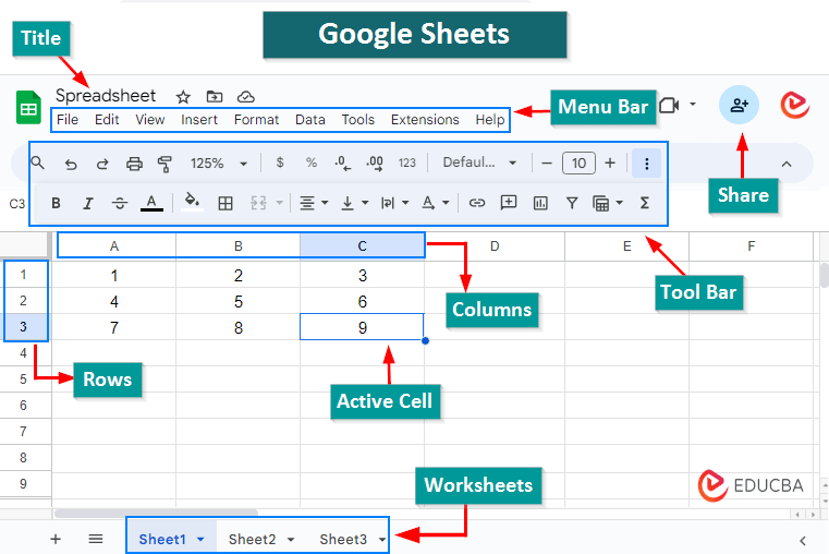
Upon opening a new spreadsheet in Google Sheets, you’ll be greeted by a familiar grid. Let’s break down the key components of this interface.

Cells, Rows, and Columns: The Building Blocks

At the heart of every spreadsheet are three fundamental elements:

Cell: This is the smallest unit of a spreadsheet, an individual box where you enter data. Each cell has a unique Cell Address defined by its column letter and row number (e.g., A1, B5, C10).
Row: A horizontal line of cells, identified by numbers (1, 2, 3…).
Column: A vertical line of cells, identified by letters (A, B, C…).

Understanding these basic components is crucial for navigating and referencing data in Google Sheets. For example, if you want to reference the cell at the intersection of column A and row 1, you’d refer to it as A1.

The Toolbar: Your Command Center

Located just below the main menu (File, Edit, View, etc.), the toolbar is packed with icons for quick access to common formatting and editing options. You’ll find tools for:

Formatting Text: Bold, Italic, Underline, Font size, Font color.
Aligning Content: Left, Center, Right, Vertical alignment.
Number Formatting: Currency, Percentage, Date, etc.
Cell Borders and Fill Color: Enhancing the visual appeal of your data.
Merge Cells, Wrap Text, Rotate Text: Controlling how text fits within cells.
Creating Filters, Charts, and Functions: More advanced operations we’ll explore.

The Formula Bar: Where the Magic Happens

Just above the column letters is the Formula Bar. This is a critical area where you can:

View the content of the currently selected cell.
Enter or edit data, text, or formulas. When you type a formula, it will appear here and the result will display in the cell itself.

Sheets (Tabs) at the Bottom

At the very bottom of your Google Sheets window, you’ll see tabs labeled “Sheet1,” “Sheet2,” and so on. These represent different worksheets within the same spreadsheet file.

Click the “+” icon to add a new sheet.
Right-click on a sheet name to Rename, Duplicate, Delete, or Hide a sheet. This is incredibly useful for organizing different datasets or reports within one file.

Essential Google Sheets Formulas for Beginners

Formulas are the beating heart of Google Sheets. They allow you to perform calculations, automate tasks, and derive insights from your data without manual effort. Every formula in Google Sheets begins with an equals sign (=).

Basic Arithmetic Operations

Let’s start with the simplest calculations, just like a calculator, but with cell references:

Addition: =A1+A2 (Adds the values in cell A1 and A2)
Subtraction: =B5-B6 (Subtracts the value in B6 from B5)
Multiplication: =C1*C2 (Multiplies values in C1 and C2)
Division: =D4/D5 (Divides the value in D4 by D5)

Practical Example: Calculating Total Items Purchased
Imagine you have a list of products and the quantity of each.
| Product | Quantity |
| :—— | :——- |
| A | 10 |
| B | 15 |
| C | 7 |

To calculate the total quantity of products A and B, you could put =B2+B3 in cell B5.

The Mighty `SUM` Function

While basic addition works for a few cells, what if you need to add hundreds or thousands? That’s where the SUM function comes in.

Purpose: Adds up a range of numbers.
Syntax: =SUM(range) or =SUM(value1, [value2, ...])
Explanation: range refers to a group of cells. For example, B2:B10 means “all cells from B2 to B10 inclusively.”
Example: To total the quantities in our example: =SUM(B2:B4) would give you 32.
- B2:B4: This is the range of cells whose values you want to add together.
Practical Use: Calculating total monthly sales, summing up all expenses for a project, or finding the grand total of inventory items.

Counting with `COUNT` and `COUNTA`

These functions help you quickly count how many cells contain certain types of data.

COUNT: Counts the number of cells in a range that contain numbers.
- Syntax: =COUNT(range)
- Practical Use: Counting how many employees submitted their numerical performance reviews.
COUNTA: Counts the number of cells in a range that are not empty (i.e., contain any type of data: numbers, text, dates).
- Syntax: =COUNTA(range)
- Practical Use: Counting the total number of entries in a client list, regardless of whether it’s a name or an ID.

Finding Averages with `AVERAGE`

The AVERAGE function calculates the arithmetic mean of a range of numbers.

Purpose: To find the typical value in a dataset.
Syntax: =AVERAGE(range)
Example: If your daily sales figures are in cells C2:C31, =AVERAGE(C2:C31) would give you the average daily sales for the month.
Practical Use: Calculating average exam scores for students, determining the average customer spend, or finding the average duration of tasks.

Finding Extremes with `MAX` and `MIN`

These functions help you quickly identify the highest and lowest values in a dataset.

MAX: Returns the largest number in a range.
- Syntax: =MAX(range)
- Practical Use: Finding the highest sales figure in a quarter, identifying the highest score on a test.
MIN: Returns the smallest number in a range.
- Syntax: =MIN(range)
- Practical Use: Determining the lowest stock level for a product, finding the lowest temperature recorded in a month.

Organizing Your Data: Sorting, Filtering, and Conditional Formatting

Raw data can be overwhelming. Google Sheets provides powerful tools to organize, clean, and highlight important information, making your data digestible and actionable.

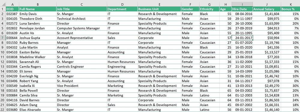
Sorting Your Data

Sorting arranges your data in a logical order, either alphabetically, numerically, or chronologically.

Select Your Data: Click and drag to select all the data you want to sort, including your header row.
Go to Data Menu: Click Data in the top menu.
Choose Sort Option:
- Sort range: For sorting specific selected data.
- Sort sheet: For sorting the entire sheet based on a column.
Configure Sort Rules: In the dialog box, ensure “Data has header row” is checked if you selected your headers. Choose the Column you want to sort by and whether you want A → Z (ascending) or Z → A (descending) order.
Click Sort: Your data will instantly reorder.

Practical Use: Sorting a customer list by last name, arranging products by price from lowest to highest, or ordering project tasks by deadline.

Filtering Your Data

Filtering allows you to temporarily hide rows that don’t meet specific criteria, letting you focus only on the relevant data.

Select Your Data: Select the range of cells you want to filter, including your header row.
Create a Filter: Go to Data > Create a filter. You’ll see small filter icons appear on each header cell.
Apply Filter: Click on a filter icon in the header of the column you want to filter by.
- You can then deselect items you don’t want to see, filter by condition (e.g., “text contains,” “number is greater than”), or filter by values (select specific items from a list).
Click OK: Only the rows matching your criteria will be displayed. The other rows are just hidden, not deleted.
Remove Filter: Go to Data > Remove filter to see all your data again.

Practical Use: Showing only sales from a specific region, viewing only tasks that are “In Progress,” or filtering a student list to see those with grades below a certain threshold.

Conditional Formatting

Conditional formatting applies specific formatting (like changing cell color or font style) to cells that meet certain conditions, making key data points instantly visible.

Select Your Range: Select the cells or range you want to apply formatting to.
Open Conditional Formatting: Go to Format > Conditional formatting. A sidebar will open.
Define Your Rule:
- Format rules: Choose a condition from the “Format rules” dropdown (e.g., “Text contains”, “Greater than”, “Date is before”).
- Value or formula: Enter the specific value or formula for your condition.
- Formatting style: Choose how you want the cells to look (e.g., fill color, text color, bold).
Click Done: The formatting will be applied dynamically. If a cell’s value changes and meets the condition, its format will update automatically.

Practical Use: Highlighting overdue tasks in red, marking sales figures above target in green, or identifying low inventory levels with a yellow background.

Visualizing Your Data: Charts and Graphs

Numbers alone can sometimes be hard to interpret. Charts and graphs turn your data into compelling visual stories, making trends, comparisons, and distributions much easier to understand.

Creating a Simple Column Chart

Column charts are excellent for comparing values across different categories.

Select Your Data: Select the range of data you want to chart. For example, select your product names and their corresponding quantities.
Insert Chart: Go to Insert > Chart. The Chart editor sidebar will appear.
Choose Chart Type: Google Sheets often intelligently suggests a chart type. If not, click on “Chart type” in the Chart editor and select Column chart.
Customize (Optional): In the Chart editor, you can customize the Chart title, Axis titles, colors, and more under the Customize tab.
Insert: The chart will appear on your spreadsheet. You can drag and resize it.

Practical Use: Comparing monthly sales performance, showing product popularity, or illustrating attendance figures over time.

Understanding Pie Charts

Pie charts are ideal for showing parts of a whole, illustrating the proportion of each category within a total.

Select Your Data: Select two columns: one for categories (e.g., “Expense Category”) and one for their corresponding values (e.g., “Amount Spent”).
Insert Chart: Go to Insert > Chart.
Choose Chart Type: In the Chart editor, select Pie chart.
Customize: Under the Customize tab, you can add data labels (percentages), change colors, and adjust the title.

Practical Use: Showing the distribution of a budget across different categories, illustrating market share for various competitors, or breaking down a company’s revenue streams.

Streamlining Workflow: Data Validation and Basic Pivot Tables

As you grow more comfortable with Google Sheets, you’ll want to ensure data accuracy and extract deeper insights. Data validation helps maintain data quality, while pivot tables summarize vast amounts of data with ease.

Data Validation: Ensuring Accuracy

Data validation restricts what can be entered into a cell, preventing errors and ensuring consistency.

Select Cells: Select the cell(s) where you want to apply data validation.
Add Validation Rule: Go to Data > Data validation > Add rule. The “Data validation rules” sidebar will open.
Choose Criteria:
- Dropdown (from a range): Create a dropdown list using values from a specific range of cells (e.g., A1:A3).
- Dropdown (custom values): Type in values directly (e.g., “High”, “Medium”, “Low”).
- Number, Text, Date: Restrict input to specific types or ranges (e.g., “Number between 1 and 100”).
- Custom formula is: For advanced validation using formulas.
Configure Action on Invalid Data:
- Show warning: Allows invalid input but displays a warning triangle.
- Reject input: Prevents invalid data from being entered.
Click Done: A dropdown arrow will appear in the selected cells, or the rule will silently enforce the input type.

Practical Use: Creating dropdowns for project statuses (“Not Started”, “In Progress”, “Completed”), ensuring that invoice numbers are always numerical, or making sure dates are within a valid range.

Introduction to Pivot Tables (Summarizing Large Datasets)

Pivot tables are incredibly powerful tools for summarizing and reorganizing large datasets to uncover trends and insights. They allow you to transform raw data into meaningful reports with just a few clicks.

Select Your Data: Select the entire range of data you want to analyze, including your header row.
Insert Pivot Table: Go to Insert > Pivot table.
Choose Destination: You can create it in a New sheet (recommended) or an existing sheet. Click Create.
Configure Pivot Table Editor: A new sheet will open with a sidebar called “Pivot table editor.” This is where the magic happens.
- Rows: Drag and drop fields (your column headers) here to display them as rows in your summary.
- Columns: Drag fields here to display them as columns.
- Values: Drag the numerical field you want to summarize (e.g., “Sales Amount,” “Quantity”) here. Google Sheets will automatically suggest a summary function like SUM or COUNT. You can change this (e.g., to AVERAGE, MAX, MIN).
- Filters: Drag fields here to filter your entire pivot table based on specific criteria (e.g., “Region = East”).

Practical Use: Summarizing total sales by product category, calculating average order value per sales representative, or analyzing the number of projects completed by different teams.

Common Google Sheets Errors and How to Fix Them

Even the most experienced data analysts encounter errors. Don’t worry, they’re part of the learning process! Here are some common Google Sheets errors and how to troubleshoot them.

`#DIV/0!` (Division by Zero)

Cause: This error occurs when a formula attempts to divide a number by zero or an empty cell.
Fix: Check your denominator! Ensure the cell referenced for division contains a non-zero number. You can also use the IFERROR function to elegantly handle potential division by zero errors, for example: =IFERROR(A1/B1, "N/A").

`#REF!` (Invalid Cell Reference)

Cause: This usually means a formula is trying to refer to a cell that no longer exists (e.g., you deleted a row or column that the formula was referencing). It can also happen when copying formulas incorrectly.
Fix:
1. Undo: If you just made a change, try pressing Ctrl+Z (Windows) or Cmd+Z (Mac) to undo.
2. Check the Formula: Click on the cell with the #REF! error and examine the formula in the Formula Bar. You’ll likely see #REF! where a valid cell reference should be. Adjust the formula to refer to the correct cells.

`#NAME?` (Unknown Function Name)

Cause: You’ve likely misspelled a function name (e.g., typing =SUMM(A1:A10) instead of =SUM(A1:A10)).
Fix: Carefully check the spelling of the function in your formula. Google Sheets’ auto-suggestion feature can help you avoid this by suggesting correct function names as you type.

`#####` (Column Not Wide Enough)

Cause: This isn’t strictly an error but a display issue. It means the number, date, or time you’ve entered is too wide to fit within the current column width.
Fix: Double-click the line between the column letter (e.g., between A and B) to automatically adjust the column width to fit the content, or drag the column border manually.

Tip: When debugging, always start by checking the formula in the Formula Bar for the problematic cell. Google Sheets will often highlight the problematic part of the formula.

Unlocking More Potential with Google Sheets

You’ve now covered the essential building blocks of Google Sheets. But this powerful tool has even more to offer:

More Advanced Functions: Explore functions like IF statements for conditional logic, VLOOKUP (or the more flexible XLOOKUP) for searching and retrieving data, ARRAYFORMULA for applying formulas to entire ranges, and QUERY for database-like operations.
Add-ons: Enhance Google Sheets with third-party add-ons from the Google Workspace Marketplace (Extensions > Add-ons > Get add-ons). These can do anything from merging cells based on conditions to connecting with other apps.
Google Apps Script: For the truly adventurous, Google Apps Script allows you to write custom code to automate tasks, create custom functions, and integrate Google Sheets with other Google services and external APIs.

Your journey with Google Sheets has just begun, and the possibilities are endless!

Conclusion: Your Journey Has Just Begun

Congratulations! You’ve just completed The Ultimate Guide to Google Sheets for Beginners. You’ve gone from understanding the basic interface to mastering essential formulas like SUM, AVERAGE, MAX, and MIN. You now know how to effectively organize your data using sorting, filtering, and conditional formatting, and how to create compelling visualizations with charts. We also touched upon crucial features like data validation for accuracy and the power of pivot tables for data summarization, along with common error troubleshooting.

Google Sheets is an incredibly versatile tool that can streamline your work, save you countless hours, and help you make data-driven decisions. Remember, the key to becoming proficient is practice. Apply what you’ve learned to your own projects, experiment with different functions, and don’t be afraid to make mistakes – that’s how we learn best. Keep exploring AskByteWise.com for more in-depth tutorials and tips to further expand your Google Sheets expertise. Happy spreading!

Frequently Asked Questions (FAQ)

Q1: Can I use Google Sheets offline?

A1: Yes! You can enable offline access for Google Drive, which includes Google Sheets. To do this, go to drive.google.com, click the Settings gear icon, select Settings, and turn on “Offline” access. This will sync your files so you can work on them without an internet connection. Changes will sync once you’re back online.

Q2: How is Google Sheets different from Microsoft Excel?

A2: While both are powerful spreadsheet applications, the main differences lie in their core nature. Google Sheets is primarily cloud-based, emphasizing real-time collaboration, automatic saving, and accessibility from any device. Excel is traditionally a desktop application, offering a more robust feature set for very large datasets and highly complex computations, though its online version has improved. For most users and typical office tasks, Google Sheets provides ample functionality and superior collaboration.

Q3: How do I share my Google Sheet with others?

A3: Sharing is one of Google Sheets’ strongest features! Click the “Share” button in the top right corner. You can then:

Enter specific email addresses to share with individuals or groups.
Set their permissions (e.g., “Viewer”, “Commenter”, “Editor”).
Click “Get link” to generate a shareable link that can be restricted to specific people or made accessible to anyone with the link (with specified permissions).

Q4: What are some good resources to learn more about Google Sheets?

A4: Beyond AskByteWise.com, which regularly publishes in-depth tutorials, you can explore:

Google’s Official Sheets Help Center: Offers comprehensive documentation.
YouTube Tutorials: Many channels provide visual, step-by-step guides.
Online Courses: Platforms like Coursera, Udemy, and LinkedIn Learning offer structured courses from beginner to advanced levels.

Q5: Is there a limit to the number of rows or columns in Google Sheets?

A5: Yes, there are limits, though they are quite generous for most users. As of my last update, a single Google Sheet can handle up to 10 million cells in total. This means you could have, for example, 10,000 rows and 1,000 columns, or 1 million rows and 10 columns. For the vast majority of personal and business needs, this limit is more than sufficient.

See more: The Ultimate Guide to Google Sheets for Beginners” by “Google Sheets.

Discover: AskByteWise.