Tired of wrestling with complex data, manually filtering rows, or struggling to create meaningful reports from your Google Sheets? Do you find yourself wishing your spreadsheet could answer questions like, “What were our top 5 best-selling products last quarter, and what was their average revenue?” If so, you’re not alone. Many office professionals and students grapple with extracting specific insights from their data without resorting to complicated workarounds or advanced programming. But what if I told you there’s a powerful, yet surprisingly intuitive function built right into Google Sheets that can transform how you interact with your data? Welcome to The QUERY Function in Google Sheets: A Complete Guide. This function is often called the “SQL of Google Sheets” because it allows you to query your data using a simple, SQL-like language, unlocking unparalleled flexibility and power for data analysis and reporting.
As your guide from AskByteWise.com, my goal is to demystify The QUERY Function in Google Sheets: A Complete Guide. We’ll break down this incredibly versatile tool, showing you how to go from raw data to insightful, dynamic reports with just a single formula. Whether you’re tracking sales, managing inventory, or analyzing survey results, mastering the QUERY function will elevate your Google Sheets game, making complex tech simple and helping you derive critical business intelligence effortlessly. Let’s dive in!
What is the QUERY Function? The SQL of Google Sheets
At its core, the QUERY function is a database query language built directly into Google Sheets. Think of it like this: instead of manually sifting through thousands of rows and columns, QUERY lets you “ask” your spreadsheet questions in a structured way. You tell it what data you want to see, what conditions that data must meet, and how you want it presented. It’s significantly more powerful than functions like FILTER, SUMIF, or even basic Pivot Tables because it combines their capabilities and more into a single, highly customizable formula.
Imagine your data as a library.
- FILTER is like asking the librarian, “Show me all books by this author.”
- SUMIF is like asking, “What’s the total page count of books by this author?”
- QUERY is like asking, “Show me the titles and average ratings of the top 10 sci-fi books published in the last year, written by authors whose names start with ‘A’, grouped by genre, and sorted by rating, but only if they have more than 500 pages.”
You see the difference? The QUERY function allows for complex, multi-criteria data extraction, aggregation, and manipulation, making it an indispensable tool for anyone who works with data in Google Sheets.
Understanding the QUERY Function Syntax
Before we unleash its full power, let’s understand the basic structure of the QUERY function.
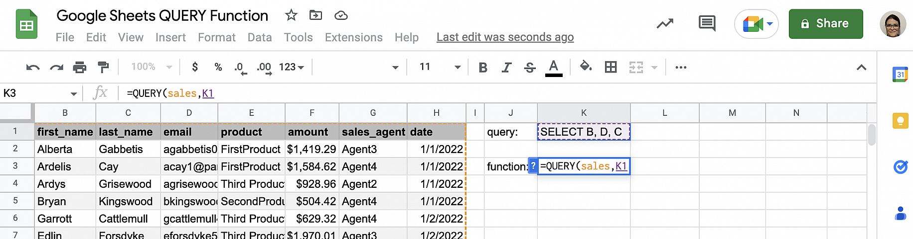
The syntax for the QUERY function is:
=QUERY(data, query, [headers])
Let’s break down each argument:
data: This is the range of cells you want to query. It’s your dataset. This could be something likeA1:E100,Sheet2!A:F, or even the output of another function likeIMPORTRANGE. It’s crucial that your data is well-structured, with each column representing a distinct category (e.g., “Product Name”, “Sales Amount”, “Date”).query: This is where the magic happens. It’s a text string, enclosed in double quotes (""), containing the SQL-like commands that tell QUERY exactly what to do. This string is comprised of one or more clauses (like SELECT, WHERE, GROUP BY, etc.), which we’ll explore in detail.[headers](Optional): This argument tells QUERY how many header rows are in yourdatarange.- If
headersis1(or omitted), QUERY treats the first row of yourdataas headers. - If
headersis0, QUERY treats all rows as data and assigns generic column labels (col1,col2, etc.). - If
headersis-1, QUERY attempts to intelligently detect the number of header rows.
In most cases, you’ll either omit it (defaulting to 1) or explicitly set it to1if you have one header row.
- If
Important Note: When referring to columns within the
querystring, you must use capital letters (e.g.,A,B,C) corresponding to the actual column letters of yourdatarange, regardless of whether your data starts in column A or D. If yourdatarange isC1:F100, then columnCin your data is referred to asCin the query,DasD, and so on. If you’re usingIMPORTRANGEor another function that returns a virtual table, columns are referred to asCol1,Col2,Col3, etc.
The Anatomy of a QUERY String (SQL-like Clauses)
The query string is where you define your data manipulation instructions. It uses a specific syntax with clauses, similar to SQL. Here are the most commonly used clauses, in their typical order:
SELECT > WHERE > GROUP BY > PIVOT > ORDER BY > LIMIT > OFFSET > LABEL > FORMAT
Let’s break down each one.
The SELECT Clause: Picking Your Columns
The SELECT clause is always the first part of your query string. It specifies which columns you want to retrieve from your data range.
- Select Specific Columns:
To select columns A, B, and D:
"SELECT A, B, D" - Select All Columns:
To select all columns in yourdatarange:
"SELECT *" - Using Aggregate Functions:
You can perform calculations on your selected columns directly withinSELECT. Common aggregate functions include:SUM(column): Calculates the total of numerical values in a column.AVG(column): Calculates the average of numerical values.COUNT(column): Counts the number of non-empty cells.MAX(column): Finds the maximum value.MIN(column): Finds the minimum value.COUNT(col1): This counts the number of non-null values in column 1. Note:COUNT(*)can also be used, butCOUNT(ColX)is generally more explicit.
Example: To get the total sales from column C:
"SELECT SUM(C)"
Example: To select product names (column A) and their total sales (column C):
"SELECT A, SUM(C)"(This usually requires aGROUP BYclause, which we’ll cover next).
The WHERE Clause: Filtering Your Data
The WHERE clause allows you to filter rows based on specific conditions. It’s how you specify which rows you want to include in your result. This clause is optional.
- Syntax:
WHERE column_name operator value - Comparison Operators:
=(Equal to)!=or<>(Not equal to)>(Greater than)<(Less than)>=(Greater than or equal to)<=(Less than or equal to)
- Logical Operators:
AND: Both conditions must be true.OR: At least one condition must be true.NOT: Negates a condition.
- Text Matching:
WHERE B = 'Electronics'(Exact match, case-sensitive). Text values must be enclosed in single quotes ('') within the query string.WHERE B CONTAINS 'phone'(Finds cells containing ‘phone’).WHERE B STARTS WITH 'App'(Finds cells starting with ‘App’).WHERE B ENDS WITH 'ice'(Finds cells ending with ‘ice’).WHERE B MATCHES '.*(phone|tablet).*'(Uses regular expressions).
- Numerical Filtering:
WHERE C > 100
WHERE D >= 50 AND D <= 200 - Date Filtering:
Dates require a specificDATE 'YYYY-MM-DD'format.
WHERE E > DATE '2023-01-01'
WHERE E >= DATE '2023-01-01' AND E <= DATE '2023-03-31'
You can also use year, month, day, quarter, etc. functions:
WHERE YEAR(E) = 2023(Note:MONTHis 0-indexed, so January is 0, February is 1, etc.)
WHERE MONTH(E) = 0(For January)
The GROUP BY Clause: Summarizing Your Data
The GROUP BY clause is used to group rows that have the same values in specified columns into a summary row. It’s often used with aggregate functions in the SELECT clause to perform calculations for each group. This is how you create summaries similar to a pivot table’s rows and values.
- Syntax:
GROUP BY column_name_1, column_name_2, ... - Example: To get the total sales (column C) for each product category (column B):
"SELECT B, SUM(C) GROUP BY B"
The PIVOT Clause: Reshaping Your Data
The PIVOT clause creates a cross-tabulation, similar to a pivot table’s columns. It transforms unique values from a specified column into new columns, summarizing values based on the GROUP BY clause.
- Syntax:
PIVOT column_to_pivot - Example: To show total sales (column C) by product category (column B), but with regions (column A) as column headers:
"SELECT B, SUM(C) GROUP BY B PIVOT A"
This creates a table with product categories as rows, regions as columns, and the sum of sales at their intersections.

*Figure 1: Example of a QUERY function using GROUP BY and PIVOT clauses to summarize sales data by product category and region, mimicking a dynamic pivot table.*
The ORDER BY Clause: Sorting Your Results
The ORDER BY clause sorts your results based on one or more columns in ascending (default) or descending order.
- Syntax:
ORDER BY column_name [ASC|DESC] - Example: To sort the previous result by total sales in descending order:
"SELECT B, SUM(C) GROUP BY B ORDER BY SUM(C) DESC"
You can sort by multiple columns:ORDER BY B ASC, SUM(C) DESC
The LIMIT and OFFSET Clauses: Paging Your Data
These clauses are used to control the number of rows returned and where to start returning them. Useful for “top N” reports or paginating large datasets.
LIMIT: Specifies the maximum number of rows to return.
"SELECT B, SUM(C) GROUP BY B ORDER BY SUM(C) DESC LIMIT 5"(Top 5 categories by sales).OFFSET: Skips a specified number of rows before returning the results.
"SELECT B, SUM(C) GROUP BY B ORDER BY SUM(C) DESC LIMIT 5 OFFSET 5"(The next 5 categories after the top 5).
The LABEL Clause: Renaming Columns
The LABEL clause allows you to assign custom, user-friendly names to the columns in your query’s output. This is especially useful when using aggregate functions, which often generate generic column names like sum C.
- Syntax:
LABEL column_name 'New Name' - Example:
"SELECT B, SUM(C) GROUP BY B LABEL B 'Product Category', SUM(C) 'Total Sales'"
The FORMAT Clause: Presenting Your Data Nicely
The FORMAT clause lets you apply specific formatting patterns to your numeric or date columns in the output.
- Syntax:
FORMAT column_name 'format_pattern' - Example: To format the total sales as currency and a date column as a specific date format:
"SELECT A, SUM(C), MAX(D) GROUP BY A LABEL SUM(C) 'Total Revenue', MAX(D) 'Last Sale Date' FORMAT SUM(C) '$#,##0.00', MAX(D) 'yyyy-MM-dd'"

*Figure 2: An example demonstrating the FORMAT clause to display currency and date values in a human-readable format directly within the QUERY output.*
Step-by-Step Examples: Putting QUERY to Work
Let’s work through some practical, business-oriented examples using a sample dataset. Imagine you have a sheet named SalesData with the following columns:
- A:
Region(e.g., “North”, “South”) - B:
Product Category(e.g., “Electronics”, “Clothing”) - C:
Product Name(e.g., “Laptop”, “T-Shirt”) - D:
Sales Amount(numerical value) - E:
Order Date(date value)
Example 1: Simple Data Extraction – Products in ‘Electronics’ Category
Let’s say you want to see all details for products belonging to the ‘Electronics’ category.
- Identify your data range:
SalesData!A:E - Formulate your query: We need to
SELECTall columns (*)WHEREtheProduct Category(column B) is'Electronics'. - Construct the QUERY function:
=QUERY(SalesData!A:E, "SELECT * WHERE B = 'Electronics'", 1)SalesData!A:E: Our data source."SELECT * WHERE B = 'Electronics'": The query string. We want all columns (*) where column B (Product Category) is exactlyElectronics.1: Indicates that our data has one header row.
Example 2: Aggregating Sales Data – Total Sales per Region, Sorted
Now, let’s calculate the total Sales Amount for each Region and then sort the results to see which regions have the highest sales.
- Identify your data range:
SalesData!A:E - Formulate your query: We need to
SELECTtheRegion(column A) and theSUMofSales Amount(column D). We’llGROUP BYRegion(column A) andORDER BYtheSUM(D)inDESCending order. - Construct the QUERY function:
=QUERY(SalesData!A:E, "SELECT A, SUM(D) GROUP BY A ORDER BY SUM(D) DESC LABEL A 'Region', SUM(D) 'Total Sales' FORMAT SUM(D) '$#,##0.00'", 1)"SELECT A, SUM(D)": Selects Region and the sum of Sales Amount."GROUP BY A": Groups the data by Region to sum sales for each."ORDER BY SUM(D) DESC": Sorts the regions from highest total sales to lowest."LABEL A 'Region', SUM(D) 'Total Sales'": Renames the output columns for clarity."FORMAT SUM(D) '$#,##0.00'": Formats theTotal Salescolumn as currency.
Example 3: Creating a Dynamic Report with Dates – Monthly Sales Growth
You want to see the total sales for a specific month and year. Let’s make this dynamic by referencing a cell for the year and month. Suppose cell G1 contains 2023 and cell G2 contains 1 (for January).
- Identify your data range:
SalesData!A:E - Formulate your query: We need
Region(A) andSUM(D),GROUP BY A. TheWHEREclause will filterOrder Date(E) by the year and month. RememberMONTHis 0-indexed. - Construct the QUERY function (using cell references with concatenation):
=QUERY(SalesData!A:E, "SELECT A, SUM(D) WHERE YEAR(E) = " & G1 & " AND MONTH(E) = " & (G2-1) & " GROUP BY A LABEL A 'Region', SUM(D) 'Monthly Sales' FORMAT SUM(D) '$#,##0.00'", 1)YEAR(E) = " & G1: Filters by the year in G1.MONTH(E) = " & (G2-1): Filters by the month in G2, adjusting for 0-indexing.- The
&(ampersand) operator is used to concatenate text strings with cell references within the query string. This is crucial for dynamic queries.
Example 4: Mimicking a Pivot Table – Sales by Product Category and Region
Let’s recreate a common pivot table scenario: total sales for each Product Category, broken down by Region.
- Identify your data range:
SalesData!A:E - Formulate your query: We want
Product Category(B),SUM(D)ofSales Amount,GROUP BY Product Category(B), and thenPIVOTbyRegion(A). - Construct the QUERY function:
=QUERY(SalesData!A:E, "SELECT B, SUM(D) GROUP BY B PIVOT A LABEL B 'Product Category'", 1)This will create a table where
Product Category(B) is in the first column, and each uniqueRegion(A) becomes a new column header, with the intersecting cells showing theSUMofSales Amountfor that category and region.
Example 5: Combining Multiple Criteria – Top 3 Products with High Sales in a Specific Category
This query will find the top 3 Product Names (C) and their total Sales Amount (D) specifically within the ‘Electronics’ Product Category (B).
- Identify your data range:
SalesData!A:E - Formulate your query:
SELECTProduct Name(C) andSUM(D),WHERE B = 'Electronics',GROUP BY Product Name(C),ORDER BY SUM(D) DESC, andLIMIT 3. - Construct the QUERY function:
=QUERY(SalesData!A:E, "SELECT C, SUM(D) WHERE B = 'Electronics' GROUP BY C ORDER BY SUM(D) DESC LIMIT 3 LABEL C 'Product Name', SUM(D) 'Total Sales' FORMAT SUM(D) '$#,##0.00'", 1)
Common Errors and How to Fix Them
Even with its power, the QUERY function can sometimes be finicky. Here are common errors and how to troubleshoot them:
#VALUE! ErrororFormula parse error:- Cause: Most often, this is due to incorrect syntax in the
querystring. This could be a missing comma, an incorrect clause order, unmatched quotes, or referring to a column incorrectly. - Fix: Carefully re-read your query string. Check for:
- All text strings (including the entire
querystring) are enclosed in double quotes ("). - All text criteria within the query string are enclosed in single quotes (
'). - Column references are capital letters (e.g.,
A,B) corresponding to the actual column of your data range. - Dates are in the
DATE 'YYYY-MM-DD'format. - Correct spelling of clauses (
SELECT,WHERE,GROUP BY, etc.). - Correct order of clauses.
- All text strings (including the entire
- Cause: Most often, this is due to incorrect syntax in the
- Dates not filtering correctly:
- Cause: Incorrect date format or comparison in the
WHEREclause. - Fix: Always use the
DATE 'YYYY-MM-DD'format for direct date comparisons. If you’re comparing against a cell reference containing a date, you’ll need to use theTEXT()function to format it correctly for the query:
"SELECT * WHERE E >= DATE '" & TEXT(G1, "yyyy-mm-dd") & "'" - Remember
MONTHis 0-indexed (Jan=0, Feb=1).
- Cause: Incorrect date format or comparison in the
- Columns referred to as
Col1,Col2in output (even if you usedA,B):- Cause: This usually happens when your
dataargument is the result of another function (likeIMPORTRANGE) or an array literal{}. In such cases, the output is a virtual table, and QUERY refers to its columns numerically. - Fix: Refer to columns in your
querystring asCol1,Col2,Col3, etc., instead ofA,B,C.
- Cause: This usually happens when your
#N/Aor blank results:- Cause: Your
WHEREclause might be too restrictive, or there’s no data matching your criteria. It could also be a case-sensitivity issue for text matching. - Fix:
- Double-check your criteria. Does the data actually exist?
- Remember text comparisons (like
WHERE B = 'Electronics') are case-sensitive. If your data has “electronics”, it won’t match “Electronics”. UseLOWER(B) = 'electronics'orUPPER(B) = 'ELECTRONICS'for case-insensitive matching if needed. - Simplify the query to isolate the problem (e.g., remove
WHEREclause, then add it back).
- Cause: Your
Tip: When building complex QUERY functions, start simple! Get the
SELECTclause working, then addWHERE, thenGROUP BY, and so on. This makes debugging much easier.
Why QUERY is a Game-Changer
The QUERY function in Google Sheets: A Complete Guide is more than just another formula; it’s a paradigm shift in how you can interact with your data.
- Unparalleled Flexibility: It combines the power of filtering, sorting, aggregating, and reshaping data into a single, cohesive command. No more nesting multiple
IF,SUMIFS,INDEX, andMATCHfunctions. - Dynamic Reports: By using cell references in your query string, you can create interactive dashboards and reports where users can change a single cell value (e.g., month, product category) and instantly update an entire report.
- Scalability: While other functions might struggle with very large datasets, QUERY is highly optimized and can efficiently process thousands, even hundreds of thousands, of rows.
- Reduced Manual Effort: Automate repetitive data extraction and summary tasks, saving you countless hours.
- SQL Skill Building: Learning QUERY is an excellent introduction to SQL, a fundamental language for database management that is highly valued in data analysis roles.
Conclusion
You’ve now embarked on a journey to master The QUERY Function in Google Sheets: A Complete Guide. From understanding its basic syntax to wielding its powerful clauses for SELECTing, WHEREing, GROUP BYing, PIVOTing, ORDER BYing, LIMITing, LABELing, and FORMATing your data, you have the knowledge to transform raw data into clear, actionable insights.
Remember, the key to becoming proficient with QUERY is practice. Start with simple queries, gradually adding more clauses and complexity. Experiment with different combinations, and don’t be afraid to make mistakes – they are your best teachers. With the QUERY function in your toolkit, you’re no longer just a spreadsheet user; you’re a data analyst, capable of extracting precise answers and building sophisticated reports with remarkable ease. Go forth and query!
Frequently Asked Questions (FAQ)
Q1: Is the QUERY function case-sensitive?
A1: Yes, by default, text comparisons in the WHERE clause (e.g., WHERE B = 'Electronics') are case-sensitive. If your data contains “electronics” (lowercase), it will not match “Electronics” (capitalized). To make queries case-insensitive, you can convert both the column and the criteria to the same case using functions like LOWER(B) = 'electronics' or UPPER(B) = 'ELECTRONICS'.
Q2: Can the QUERY function work across multiple sheets or even different Google Sheets files?
A2: Yes!
- Multiple sheets in the same file: You can reference ranges from other sheets directly, e.g.,
=QUERY(Sheet2!A:E, "SELECT *", 1). - Different Google Sheets files: You can use the
IMPORTRANGEfunction within thedataargument ofQUERY. For example:=QUERY(IMPORTRANGE("your_spreadsheet_url", "Sheet1!A:E"), "SELECT Col1, Col2 WHERE Col3 > 100", 1). Remember to useCol1, Col2, etc., whenIMPORTRANGEis the data source.
Q3: What’s the main difference between QUERY and FILTER?
A3:
- FILTER is simpler and primarily used for extracting rows that meet specific conditions. It cannot aggregate data (like
SUMorCOUNT) or reshape it (likeGROUP BYorPIVOT) on its own. - QUERY is much more powerful and versatile. It can filter, select specific columns, perform aggregations, group data, pivot data, sort, limit results, and format them, all within a single formula. If you need anything beyond basic row filtering,
QUERYis the way to go.
Q4: How do I refer to a header row in the QUERY string itself?
A4: You don’t directly refer to the header row content within the query string. Instead, the headers argument in =QUERY(data, query, [headers]) tells QUERY which row(s) to treat as headers in the output. Within the query string, you always refer to columns by their capital letter (e.g., A, B) or Col1, Col2 if your data source is virtual (like IMPORTRANGE). The LABEL clause is used to rename columns in the output if the automatically generated names aren’t suitable.
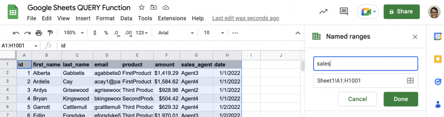
*Figure 3: An illustration of using cell references within a QUERY string, dynamically updating the filtering criteria for a report.*
Q5: Can I use cell references in the QUERY string to make it dynamic?
A5: Absolutely, and this is one of QUERY‘s most powerful features! You achieve this by breaking up your query string and concatenating (&) your cell references into it.
Example: If cell A1 contains 'Electronics' and you want to filter by that category:
=QUERY(SalesData!A:E, "SELECT * WHERE B = '" & A1 & "'", 1)
Notice the combination of double quotes for the text parts of the query string, single quotes around the cell reference for text criteria ('" & A1 & "'), and the ampersand (&) to join them. This allows your query to adapt based on values in other cells.
See more: The QUERY Function in Google Sheets: A Complete Guide.
Discover: AskByteWise.