Ever stared at a Google Sheet, only to be met with a sea of angry red error messages like #N/A or #REF!? You’re not alone. These little digital roadblocks can turn a simple task into a frustrating puzzle, making your carefully crafted reports look unprofessional and your data unreliable. But what if I told you that most of these errors are easily fixable, and understanding them is a superpower in itself? At AskByteWise, our mission is “Making Complex Tech Simple,” and today, we’re going to demystify these common Google Sheets errors. This definitive guide will equip you with the knowledge to troubleshoot and prevent the most common errors in Google Sheets, specifically tackling #N/A and #REF!, empowering you to regain control of your spreadsheets and ensure your data always tells the right story.
Understanding Google Sheets Errors: More Than Just Red Text
Think of Google Sheets errors as your spreadsheet’s way of telling you, “Hey, something isn’t quite right here!” They’re not there to punish you, but rather to alert you to a logical or data integrity issue. Ignoring them can lead to incorrect calculations, flawed analyses, and ultimately, poor business decisions. For data analysts, project managers, or students working on assignments, understanding these error codes is crucial. It’s about maintaining clean data, ensuring your formulas work as intended, and building robust spreadsheets that stand up to scrutiny.
Errors usually stem from one of three areas:
- Logic Errors: Your formula is asking for something that doesn’t exist or isn’t possible (e.g., looking for a value that isn’t there).
- Data Errors: The data your formula relies on is incorrect, missing, or in the wrong format.
- Reference Errors: Your formula is pointing to a cell, range, or sheet that no longer exists or has been moved.
By breaking down the most common culprits, we can turn frustration into a clear path forward, making your journey with Google Sheets smoother and more productive.
The Infamous #N/A Error: When Google Sheets Can’t Find What It’s Looking For
The #N/A error is perhaps one of the most frequently encountered and, for many, the most puzzling. It simply means “Not Available” or “No Match Found.” If you’re using lookup functions extensively, you’ve definitely crossed paths with this one.
What Does #N/A Mean?
When you see #N/A, it’s usually because a lookup function like VLOOKUP, MATCH, XLOOKUP (which functions similarly to VLOOKUP or INDEX MATCH in Sheets), or LOOKUP can’t find the value you’re asking it to search for within the specified range. Imagine you’re asking a librarian for a book title, and they tell you it’s “Not Available” – either they don’t have it, or you gave them the wrong title. That’s essentially what #N/A is in a spreadsheet.
Common Causes of #N/A Errors
Understanding the root cause is the first step to fixing the #N/A error. Here are the most common scenarios:
-
Mismatch in Lookup Values:
- Typos: A slight misspelling in your lookup value (e.g., “Applle” instead of “Apple”).
- Extra Spaces: Leading or trailing spaces (e.g., “Apple ” instead of “Apple”) are invisible but distinct characters.
- Case Sensitivity: While VLOOKUP is generally not case-sensitive for exact matches, other functions or data sources might be.
-
Lookup Range Does Not Include the Lookup Column:
- This is a classic VLOOKUP pitfall. The value you’re searching for must be in the first column of your specified
range. If it’s not, VLOOKUP won’t find it.
- This is a classic VLOOKUP pitfall. The value you’re searching for must be in the first column of your specified
-
Data Type Mismatch:
- You might be looking for a number (e.g., product ID “123”) in a column where that product ID is stored as text (“123”). Even though they look identical, Sheets treats them differently.
-
Search Key Not Existing in the Lookup Array:
- The most straightforward reason: the value you’re searching for genuinely isn’t present in the data you’re searching through.
-
IMPORTRANGEIssues:- If your lookup function relies on data brought in by IMPORTRANGE, issues with the
IMPORTRANGEfunction itself (incorrect URL, sheet name, range, or permissions) can lead to #N/A in the dependent formulas.
- If your lookup function relies on data brought in by IMPORTRANGE, issues with the
Step-by-Step Solutions to Fix #N/A Errors
Let’s walk through how to systematically troubleshoot and resolve #N/A errors.
1. Check Your Lookup Value and Range
This is often the quickest fix.
- Identify the problematic cell showing #N/A.
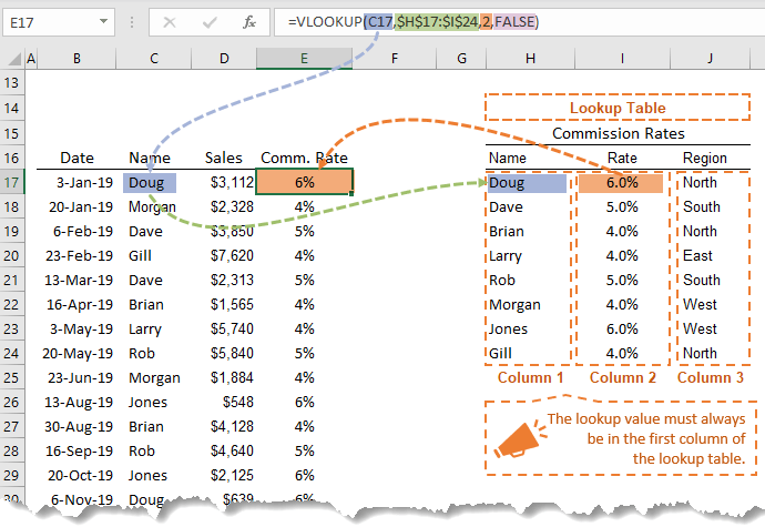
- Examine the formula in that cell. For a VLOOKUP formula like
=VLOOKUP(A2, B:C, 2, FALSE):A2is your lookup value. Is it typed correctly?B:Cis your range. Is the value in A2 definitely in column B (the first column of your range)?
- Clean your data:
- Remove extra spaces: Use the TRIM function on both your lookup value and the lookup column data.
- For example, if your lookup value is in A2, try
=TRIM(A2)in a temporary cell to see the cleaned version. - To clean the whole column B, you might copy column B to a new column (say D), use the formula
=ARRAYFORMULA(TRIM(B:B))in cell D1, then copy and paste special (values only) back to column B if necessary.
- For example, if your lookup value is in A2, try
- Remove extra spaces: Use the TRIM function on both your lookup value and the lookup column data.
- Verify the lookup column: For VLOOKUP, ensure the column containing the value you’re searching for is indeed the first column of the
rangeargument. If not, adjust your range or consider using INDEX MATCH.
2. Data Type Consistency
Numbers formatted as text, or text that looks like numbers, can cause mismatches.
- Select the lookup column (e.g., B) and the column containing your lookup value (e.g., A).
- Go to Format > Number > Automatic. This often helps Google Sheets correctly interpret data types.
- Use the
VALUEfunction: If you suspect a number is stored as text, wrap it inVALUE.- For example, if cell A2 has “123” as text,
=VALUE(A2)will convert it to the number 123. - You might need to create a helper column or embed
VALUEwithin your lookup function:
=VLOOKUP(VALUE(A2), B:C, 2, FALSE)(if A2 is text but B is numbers)
=VLOOKUP(A2, ARRAYFORMULA(VALUE(B:B)), 2, FALSE)(if B is text but A2 is number)
Note:ARRAYFORMULA(VALUE(B:B))is powerful but should be used cautiously on large datasets as it re-evaluates the entire column.
- For example, if cell A2 has “123” as text,
3. Ensure Lookup Key Exists
Sometimes the simplest explanation is the right one: the value isn’t there.
- Visually scan: Manually look for your lookup value (e.g., A2) in the lookup column (e.g., B).
- Use
COUNTIFto verify presence: In an empty cell, type=COUNTIF(B:B, A2).- If it returns
0, your value truly isn’t in column B. - If it returns
1or more, then you likely have a data type or space issue (go back to steps 1 and 2).
- If it returns
4. Using IFNA or IFERROR to Handle #N/A Gracefully
Instead of ugly #N/A messages, you can display something more user-friendly, like “Not Found” or a blank cell.
-
IFNAFunction (Specific to #N/A):- Syntax:
=IFNA(value, value_if_na) value: Your original formula that might return #N/A.value_if_na: What you want to display if #N/A occurs.- Example: If your formula is
=VLOOKUP(A2, B:C, 2, FALSE), wrap it:
=IFNA(VLOOKUP(A2, B:C, 2, FALSE), "Product Not Found") - This will show “Product Not Found” instead of #N/A. For a blank cell, use
"".
=IFNA(VLOOKUP(A2, B:C, 2, FALSE), "")
- Syntax:
-
IFERRORFunction (Catches Any Error):- Syntax:
=IFERROR(value, value_if_error) value: Your original formula.value_if_error: What you want to display if any error occurs (not just #N/A).- Example:
=IFERROR(VLOOKUP(A2, B:C, 2, FALSE), "Data Processing Error") - When to use
IFNAvs.IFERROR:IFNAis generally preferred when you specifically expect and want to handle #N/A errors, as it allows other error types (like #DIV/0!) to show, which might indicate different problems.IFERRORis a broader catch-all.
- Syntax:
5. Advanced: INDEX MATCH as a Robust Alternative
While not directly fixing #N/A related to missing values, INDEX MATCH offers more flexibility than VLOOKUP and is often less prone to certain #N/A causes (like the lookup column not being the first). It’s also often more efficient for large datasets.
- How it works:
MATCHfinds the row number of your lookup value in a specific column.INDEXthen retrieves a value from a specific row and column.
- Example: To achieve the same as
=VLOOKUP(A2, B:C, 2, FALSE):
=INDEX(C:C, MATCH(A2, B:B, 0))MATCH(A2, B:B, 0): Finds the row number where A2 is found in column B (the0ensures an exact match).INDEX(C:C, ...): Retrieves the value from column C at that specific row number.
- Handling #N/A with
INDEX MATCH: You can still wrap it inIFNAorIFERRORjust like aVLOOKUP.
=IFNA(INDEX(C:C, MATCH(A2, B:B, 0)), "Value not found")
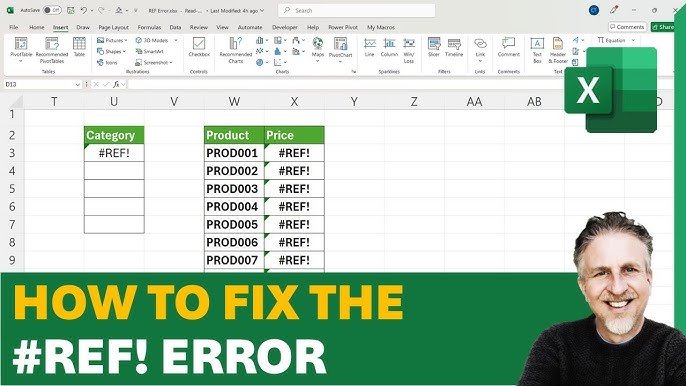
The Troublesome #REF! Error: When Your References Break Down
The #REF! error is another common one, signaling that a formula refers to an invalid cell. This error is often more severe because it indicates a structural problem within your spreadsheet, not just a data lookup issue. Think of it like a house address that no longer exists because the street was demolished.
What Does #REF! Mean?
#REF! stands for “Invalid Cell Reference.” Google Sheets is telling you that a formula is trying to refer to a cell, range, or even an entire sheet that it can no longer find. This usually happens when something that a formula was pointing to has been deleted, cut, or otherwise removed.
Common Causes of #REF! Errors
The #REF! error is almost always caused by a structural change to your spreadsheet.
-
Deleting Rows or Columns:
- If your formula refers to a cell in a row or column that you then delete, the formula loses its reference. For example, if
=SUM(A1:A5)exists, and you delete row 3, the formula might become=SUM(A1:#REF!:A4).
- If your formula refers to a cell in a row or column that you then delete, the formula loses its reference. For example, if
-
Cutting and Pasting Cells, Ranges, or Sheets:
- If you cut a cell or range that is referenced by a formula and paste it elsewhere, the original reference becomes invalid. Copying and pasting values (rather than cutting) is generally safer.
- Moving an entire sheet tab that another sheet’s formula refers to can also cause #REF!.
-
IMPORTRANGEIssues (Again):- If an
IMPORTRANGEformula is incorrect (wrong spreadsheet ID, misspelled sheet name, invalid range), any formula that then refers to the results of thatIMPORTRANGEmight display #REF!. This is because the imported data is “missing.”
- If an
-
Circular References:
- Less common, but if a formula refers back to itself, directly or indirectly, it can sometimes lead to #REF! (though often Google Sheets will flag a “circular dependency detected” warning).
Step-by-Step Solutions to Fix #REF! Errors
Fixing #REF! often involves careful inspection and, sometimes, reverting recent changes.
1. Undo Your Last Actions
This is your first line of defense! If you’ve just performed an action (like deleting rows/columns, cutting cells) and suddenly see #REF!, immediately hit Ctrl + Z (Windows) or Cmd + Z (Mac) to undo. Google Sheets also has a robust File > Version history feature that allows you to revert to an earlier state of your spreadsheet.
2. Inspect the Formula and Its References
- Select the cell showing #REF!.
- Look at the formula bar. Google Sheets will often highlight the broken part of the reference within the formula, or the error itself will appear where the broken reference should be.
- Example:
=A1 + #REF!clearly shows where the problem lies.
- Example:
- Manually correct the reference: If you know what cell or range should be referenced, simply edit the formula to correct it. For example, if it became
#REF!after deleting column C, and it was supposed to refer toB5, manually change it toB5.
3. Avoid Deleting Referenced Cells/Rows/Columns Recklessly
Prevention is key!
- Be cautious when deleting: Before deleting any row or column, consider if other formulas in your spreadsheet might be using data from it. There isn’t a direct “Show Dependents” feature like in Excel, so you need to be vigilant.
- Copy vs. Cut: When moving data, always Copy (Ctrl+C / Cmd+C) and Paste values only (Ctrl+Shift+V / Cmd+Shift+V) rather than Cut (Ctrl+X / Cmd+X) if there’s a chance other formulas might reference the original location. Cutting moves the data and often breaks references.
4. Review IMPORTRANGE Formulas
If your #REF! error stems from an IMPORTRANGE call:
- Check Spreadsheet ID: Ensure the
spreadsheet_id(the long string in the Google Sheet’s URL) is correct. - Check Sheet Name and Range: Verify that the
range_stringargument (e.g.,"Sheet1!A1:B10") correctly specifies the sheet name and range. Pay attention to spelling and exclamation marks. - Permissions: When you first use
IMPORTRANGEto a new sheet, Google Sheets will prompt you to “Allow access.” If this wasn’t done, or permissions were revoked, the formula will fail. Click the cell with theIMPORTRANGEformula and look for the “Allow access” button/prompt.
=IMPORTRANGE("1AbcDeFgHiJkLmNoPqRsTuVwXyZ012345", "SalesData!A1:D100")
5. Understanding Absolute References ($) for Stability
While absolute references don’t prevent #REF! from deletion, they are crucial for maintaining formula integrity when copying or moving formulas within a sheet.
- Relative vs. Absolute:
A1is a relative reference. If you drag a formula referring toA1down a row, it becomesA2.$A$1is an absolute reference. It will always refer to cell A1, no matter where you copy or drag the formula.$A1(column absolute, row relative) andA$1(column relative, row absolute) are mixed references.
- Use Case: If your formula refers to a specific fixed cell (like a tax rate in B1) that shouldn’t change when you copy the formula, use
$B$1. This helps prevent errors related to incorrect cell references when formulas are moved or filled.
=C2 * $B$1(calculates C2 multiplied by the fixed tax rate in B1).
Other Common Google Sheets Errors and Quick Fixes
While #N/A and #REF! are the most common, you might encounter other error messages. Here’s a quick rundown of them and how to tackle them.
#DIV/0! (Division by Zero)
- Meaning: You are trying to divide a number by zero or an empty cell (which Sheets treats as zero in calculations).
- Common Cause: A divisor in your formula is
0or blank. - Fix:
- Check the divisor: Ensure the cell being used as the divisor contains a non-zero number.
- Use
IFERRORorIF: Wrap your division formula to handle this gracefully.
=IFERROR(A1/B1, 0)(returns0if B1 is0or empty)
=IF(B1=0, "N/A", A1/B1)(returns “N/A” if B1 is0, otherwise performs division)
#VALUE! (Incorrect Argument Type or Operation)
- Meaning: A function or formula is receiving the wrong type of argument (e.g., text where it expects a number) or performing an invalid operation.
- Common Cause:
- Using text in a mathematical operation:
=A1 + B1where B1 contains “Hello”. - A function requires a number, but you’ve provided text.
- Using text in a mathematical operation:
- Fix:
- Check data types: Ensure all cells involved in calculations or function arguments are of the correct type (numbers for calculations, dates for date functions, etc.).
- Use
VALUEorN: Convert text to numbers where appropriate.VALUE("123")becomes123.N("Text")becomes0. - Inspect function arguments: Read the function’s help text (
=SUM(and then look at the tooltip) to understand what kind of arguments it expects.
#NAME? (Unknown Name/Function)
- Meaning: Google Sheets doesn’t recognize something in your formula, usually a function name or a named range.
- Common Cause:
- Misspelled function name:
=SUMM(A1:A10)instead of=SUM(A1:A10). - Misspelled named range: You’re using a named range like
SalesData, but you’ve typedSaleData. - Using a function that doesn’t exist in Google Sheets (e.g., an Excel-specific function).
- Misspelled function name:
- Fix:
- Double-check spelling: Carefully review the function name or named range in your formula.
- Use the function wizard: When you start typing a function, Sheets often suggests completions. Use these.
- Verify named ranges: Go to Data > Named ranges to ensure your named range exists and is spelled correctly.
#NUM! (Invalid Numeric Value)
- Meaning: A formula has produced a numeric value that is too large or too small to be represented, or a function that requires a numeric input has been given an invalid one (e.g., calculating the square root of a negative number).
- Common Cause:
- Mathematical operations resulting in excessively large or small numbers.
- Invalid arguments to mathematical functions (e.g.,
=SQRT(-5)). - Iterative calculations not converging.
- Fix:
- Check input values: Ensure that inputs to functions like
SQRT,LOG, etc., are valid. - Review complex calculations: Break down long formulas into smaller parts to isolate where the invalid number might be generated.
- Check input values: Ensure that inputs to functions like
#ERROR! (Generic Parsing Error)
- Meaning: This is a catch-all error, indicating a general syntax issue in your formula that Sheets can’t categorize more specifically.
- Common Cause:
- Unmatched parentheses: Forgetting a closing parenthesis.
- Missing commas or operators:
A1 B1instead ofA1+B1or=SUM(A1:A10 A2:A20)instead of=SUM(A1:A10, A2:A20). - Incorrect range syntax.
- Fix:
- Carefully review formula syntax: Look for missing commas, incorrect operators, or unbalanced parentheses. Google Sheets often highlights pairs of parentheses when you click near them, which can help.
- Build the formula step-by-step: Start with a simple version and add components one by one to see where the error appears.

Proactive Spreadsheet Habits to Prevent Errors
An ounce of prevention is worth a pound of cure. Adopting these habits can significantly reduce the occurrence of errors.
- Data Validation: Use Data > Data validation to enforce rules on what can be entered into cells (e.g., only numbers, specific items from a list, valid dates). This prevents incorrect data entry that can lead to #VALUE! or #N/A.
- Use Named Ranges: Instead of using
A1:B10, create a named range (e.g.,ProductList) via Data > Named ranges. This makes formulas more readable (=VLOOKUP(item, ProductList, 2, FALSE)) and less prone to errors if you accidentally extend or shrink a range, though care is still needed if columns are deleted. - Break Down Complex Formulas: If you have a very long, nested formula, break it into smaller, manageable parts in helper columns. This makes debugging much easier. Once debugged, you can always nest them back together.
- Add Comments: Use Insert > Comment to explain complex formulas or specific data entries. This is invaluable for collaboration and for your future self.
- Leverage Version History: Regularly check File > Version history > See version history to save snapshots of your spreadsheet. This allows you to revert to an earlier, error-free version if something goes wrong.
- Test Formulas with Sample Data: Before applying a formula to a massive dataset, test it on a small, controlled sample to ensure it behaves as expected.
- Structure Your Data: Keep your data organized in tables, with clear headers. Avoid blank rows or columns within your data sets, especially when using functions that expect contiguous ranges.
Conclusion: Master Your Data, Master Your Workflow
Facing Google Sheets errors like #N/A and #REF! can be daunting, but as Noah Evans from AskByteWise, I hope this comprehensive guide has shown you that they are not insurmountable obstacles. By understanding what these errors mean, knowing their common causes, and applying the step-by-step solutions we’ve covered, you’re not just fixing a spreadsheet; you’re developing critical data literacy skills.
Remember, every error message is a learning opportunity. It’s Google Sheets giving you feedback, guiding you toward more robust formulas and cleaner data. By adopting proactive habits and confidently troubleshooting, you’ll transform your relationship with spreadsheets, making them powerful tools for analysis and productivity. Keep practicing, keep exploring, and keep making complex tech simple. Your data, and your workflow, will thank you for it!
Frequently Asked Questions (FAQ)
Q1: Can I make all errors show “0” instead of the error message?
A: Yes, you can use the IFERROR function. Wrap your formula with IFERROR(your_formula, 0). For example, =IFERROR(VLOOKUP(A2, B:C, 2, FALSE), 0) will return 0 if the VLOOKUP results in any error. While useful, be mindful that it hides all error types, so you might miss other potential issues besides #N/A.
Q2: Why does my VLOOKUP return #N/A even when the value is clearly there?
A: This is extremely common! The usual culprits are:
- Leading/Trailing Spaces: The lookup value or values in the lookup column have invisible extra spaces. Use the TRIM function to clean them.
- Data Type Mismatch: One side is a number, the other is text. Use
VALUE()or Format > Number > Automatic to standardize. - Case Sensitivity (less common for VLOOKUP exact match): While
VLOOKUPwithFALSE(exact match) is generally not case-sensitive, ensure consistency. - Lookup Column Not First: For
VLOOKUP, the value you’re searching for must be in the first column of your specifiedrange. If it’s not, it won’t be found.
Q3: What’s the best way to avoid #REF! errors when collaborating?
A: Communication is key! Always notify collaborators before making structural changes like deleting rows/columns or moving sheets. Additionally:
- Use absolute references (
$) for fixed cells in formulas. - Avoid cutting data; instead, copy and paste values if you need to move data.
- Regularly save version history to easily revert if an error occurs.
- Consider sheet protection for critical areas to prevent accidental deletions.
Q4: Is IFNA better than IFERROR?
A: It depends on your specific needs.
IFNAis more precise: It only catches #N/A errors. This is beneficial when you specifically expect #N/A due to a lookup not finding a value, but you want other errors (like #DIV/0! or #VALUE!) to remain visible, as they might indicate different underlying problems.IFERRORis a catch-all: It hides any error type. While convenient for making a sheet look clean, it can mask critical errors that you might want to investigate.
Recommendation: UseIFNAwhen you specifically expect an #N/A; useIFERRORif you want a general cleaner output and are confident other errors won’t be a problem.
Q5: How do I find all cells with errors in a large Google Sheet?
A: There are a couple of quick ways:
- Conditional Formatting: Select your entire data range. Go to Format > Conditional formatting. Under “Format rules,” choose “Custom formula is” and enter a formula like
=ISERROR(A1). Set a distinct fill color (e.g., bright red) to highlight all cells with errors. - Filter by Condition: Select your entire dataset, then go to Data > Create a filter. Click the filter icon on any column header, choose “Filter by condition,” then select “Custom formula is” and enter
=ISERROR(A1)(replacingA1with the first cell of that specific column). This will filter your sheet to show only rows containing errors in that column. You can repeat for other columns.
See more: How to Fix the Most Common Errors in Google Sheets (#N/A, #REF!).
Discover: AskByteWise.