Mastering VLOOKUP: A Beginner’s Step-by-Step Guide

Tired of manually sifting through endless spreadsheets, trying to match data points from one list to another? You’re not alone. Many office professionals and students grapple with this common data challenge daily. But what if there was a powerful tool that could automate this tedious process for you, saving hours and eliminating errors? Enter VLOOKUP, a fundamental function in spreadsheet software like Microsoft Excel and Google Sheets that allows you to efficiently find specific information in large datasets. This comprehensive guide, “Mastering VLOOKUP: A Beginner’s Step-by-Step Guide,” will demystify this essential function, breaking down its components and showing you exactly how to wield its power, transforming you into a spreadsheet wizard.

What Exactly is VLOOKUP, and Why Should You Care?

Imagine you’re at a library. You have the title of a book, and you want to find out its genre, author, and shelf location. You wouldn’t browse every single shelf; you’d go to the catalog, look up the book title, and then the catalog would tell you where to find it.

VLOOKUP works much the same way within your spreadsheet. The “V” stands for “Vertical,” meaning it looks for data vertically down the first column of a specified table, and then returns a value from a different column in the same row. It’s your personal spreadsheet data librarian!

Why is this so important?

• Saves Time: No more manual copying and pasting data from one sheet to another based on a common identifier.
• Reduces Errors: Human error is inevitable with manual lookups. VLOOKUP provides consistent, accurate results.
• Enhances Data Analysis: Quickly pull related data to enrich your reports, such as matching product IDs to their sales figures, or employee IDs to their department names.
• Boosts Productivity: Free up valuable time for more analytical and strategic tasks.

Whether you’re calculating monthly sales growth, cross-referencing customer orders, or compiling student grades, VLOOKUP is an indispensable skill for anyone working with data.

Deconstructing the VLOOKUP Formula: The Four Essential Arguments

Every powerful tool has its components, and VLOOKUP is no different. The formula might look intimidating at first, but once we break down its four core pieces (called “arguments”), you’ll see how simple it truly is.

Here’s the basic syntax for the VLOOKUP function:

=VLOOKUP(lookup_value, table_array, col_index_num, [range_lookup])

Let’s dissect each part:

1. lookup_value (What are you looking for?)

   • This is the specific piece of data you want to find. Think of it as the “book title” in our library analogy.
   • It could be a product ID, an employee number, a customer name, or any unique identifier.
   • You’ll usually reference a cell containing this value (e.g., A2).

2. table_array (Where are you looking for it?)

   • This is the entire range of cells where your data is located. It’s the “catalog” in our analogy.
   • It must include both the lookup_value (which must be in the first column of this range) and the value you want to retrieve.
   • When referencing this range, it’s crucial to use absolute references (e.g., $A$1:$D$100) if you plan to drag the formula down. This prevents the range from shifting.

3. col_index_num (Which column contains the answer?)

   • This is a number representing the column position within your table_array that contains the data you want to return.
   • The first column of your table_array is always 1, the second is 2, and so on.
   • Important: This is not the column number on the entire spreadsheet (e.g., column C isn’t always 3). It’s relative to your selected table_array.

4. [range_lookup] (Exact match or approximate match?)

   • This is an optional argument, indicated by the square brackets, but it’s critically important. It tells VLOOKUP how precisely you want to match your lookup_value.
   • FALSE (or 0): This specifies an exact match. VLOOKUP will only find the exact lookup_value you’ve provided. If it can’t find it, it returns an #N/A error. This is the most common and safest option for most situations.
   • TRUE (or 1): This specifies an approximate match. VLOOKUP will look for an exact match, but if it doesn’t find one, it will return the closest value that is less than or equal to your lookup_value. This requires the first column of your table_array to be sorted in ascending order. We’ll explore this later.

Tip: For beginners, always start with FALSE for the range_lookup argument unless you explicitly understand and need an approximate match. This prevents unexpected results.

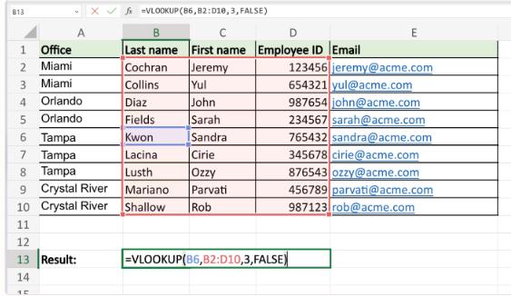
Here’s a visual representation of how these arguments map to your spreadsheet data:

Step-by-Step: Your First VLOOKUP Formula (Exact Match)

Let’s put theory into practice with a common business scenario: matching product IDs to their corresponding product names.

Scenario: Linking Product IDs to Product Names

Imagine you have a list of sales transactions with only Product IDs, but you need to add the Product Name for each sale from a separate product catalog.

Dataset 1: Sales Transactions (where we want to add Product Name)

Sales ID	Product ID	Quantity
1001	P105	10
1002	P102	5
1003	P107	12
1004	P101	8
1005	P102	3

Dataset 2: Product Catalog (where the product names are stored)

Product ID	Product Name	Category	Unit Price
P101	Laptop	Electronics	1200
P102	Mouse	Accessories	25
P103	Keyboard	Accessories	75
P104	Monitor	Electronics	300
P105	Webcam	Accessories	50
P106	Printer	Peripherals	150
P107	Headphones	Audio	100

Our goal is to populate a new “Product Name” column in Dataset 1 using the Product ID as our common link.

Let’s assume:

• Dataset 1 is on Sheet1, starting in A1.
• Dataset 2 is on Sheet2, starting in A1.
• We want the Product Name to appear in cell D2 of Sheet1 for the first sales entry.

1. Prepare Your Data

Ensure your data is clean and consistent. Make sure the lookup_value (Product ID in Dataset 1) and the first column of your table_array (Product ID in Dataset 2) have the exact same format (e.g., no extra spaces, consistent capitalization if case-sensitive, though VLOOKUP is generally not case-sensitive).

2. Identify Your lookup_value

For the first sales entry (Sales ID 1001), our lookup_value is P105. This is located in cell B2 on Sheet1.

• lookup_value = B2

3. Define Your table_array

We need to search for P105 in Dataset 2. The table_array must start with the column containing the lookup_value (Product ID) and extend to include the column with the data we want to retrieve (Product Name).

On Sheet2, our data ranges from A2 (Product ID “P101”) to D8 (Unit Price “100”).
So, our table_array will be Sheet2!A2:D8.

Important Note: When copying formulas, cell references can shift. To prevent your table_array from changing as you drag your formula down, make it an absolute reference using dollar signs ($).

• table_array = Sheet2!$A$2:$D$8

4. Determine Your col_index_num

We want to retrieve the Product Name. In our table_array (Sheet2!$A$2:$D$8):

• Column A (Product ID) is column 1.
• Column B (Product Name) is column 2.
• Column C (Category) is column 3.
• Column D (Unit Price) is column 4.

Since we want the Product Name, our col_index_num is 2.

• col_index_num = 2

5. Set Your range_lookup

We need an exact match for the Product ID (e.g., P105 must find P105, not P104). So, we’ll use FALSE.

• range_lookup = FALSE

6. Assemble the Formula

Now, let’s put all the pieces together in cell D2 on Sheet1:

=VLOOKUP(B2,Sheet2!$A$2:$D$8,2,FALSE)

After typing this formula and pressing Enter, cell D2 on Sheet1 should display “Webcam”.

7. Drag and Fill

To apply this formula to the rest of your sales transactions, simply click on cell D2, then click and drag the small square (the fill handle) at the bottom-right corner of the cell downwards. VLOOKUP will automatically populate the Product Names for all corresponding Product IDs.

Here’s how Sheet1 would look after applying the formula:

Sales ID	Product ID	Quantity	Product Name
1001	P105	10	Webcam
1002	P102	5	Mouse
1003	P107	12	Headphones
1004	P101	8	Laptop
1005	P102	3	Mouse

Congratulations! You’ve just performed your first successful VLOOKUP. This is a powerful technique for anyone managing sales data, customer records, or inventory.

VLOOKUP for Approximate Matches: When “Close Enough” is Good Enough

While exact matches are most common, VLOOKUP can also handle approximate matches. This is incredibly useful for scenarios involving ranges, such as grading systems, commission tiers, or tax brackets.

For approximate matches, you use TRUE (or 1) for the range_lookup argument:

=VLOOKUP(lookup_value, table_array, col_index_num, TRUE)

Crucial Rule for Approximate Match: Sorted Data

The most critical requirement for an approximate VLOOKUP is that the first column of your table_array must be sorted in ascending order. If it’s not, your results will be incorrect.

Scenario: Assigning Letter Grades Based on Scores

Let’s say you have a list of student scores and you need to assign them a letter grade based on the following scale:

Grading Scale (our table_array)

Minimum Score	Grade
0	F
60	D
70	C
80	B
90	A

Student Scores (where we want to add the Grade)

Student Name	Score
Alice	75
Bob	92
Carol	68
David	55
Eve	80

Let’s assume the Student Scores are on Sheet1 starting at A1, and the Grading Scale is on Sheet2 starting at A1. We want the grade for Alice (score 75) in cell C2 on Sheet1.

1. Ensure table_array is Sorted: Our Grading Scale (Sheet2!A2:B6) is sorted by “Minimum Score” in ascending order (0, 60, 70, 80, 90). Perfect!

2. Identify lookup_value: For Alice, her score is 75, in cell B2 on Sheet1.

   • lookup_value = B2

3. Define table_array: Our grading scale is Sheet2!A2:B6. Remember to use absolute references if dragging down.

   • table_array = Sheet2!$A$2:$B$6

4. Determine col_index_num: We want the “Grade,” which is in the second column of our table_array.

   • col_index_num = 2

5. Set range_lookup: We need an approximate match here. A score of 75 should fall into the “C” range (since it’s between 70 and 80).

   • range_lookup = TRUE

6. Assemble the Formula: In cell C2 on Sheet1:

   =VLOOKUP(B2,Sheet2!$A$2:$B$6,2,TRUE)

   Press Enter. Cell C2 should now display “C”.

7. Drag and Fill: Drag the formula down to get the grades for Bob, Carol, David, and Eve.

Here’s how Sheet1 would look:

Student Name	Score	Grade
Alice	75	C
Bob	92	A
Carol	68	D
David	55	F
Eve	80	B

Notice how VLOOKUP found “C” for 75, “A” for 92, and “D” for 68. For 80, it found “B” because 80 is an exact match to the “Minimum Score” column. For 55, it found “F” because 55 is greater than or equal to 0, but less than 60. This demonstrates the power of approximate match for tiered data.

Common VLOOKUP Errors and How to Fix Them

Even experienced data analysts encounter errors. Understanding common VLOOKUP errors will save you a lot of frustration.

1. #N/A (Not Available)

This is the most common VLOOKUP error. It means VLOOKUP couldn’t find the lookup_value in the first column of your table_array.

Common Causes and Solutions:

• lookup_value not found: The item simply doesn’t exist in your table_array.
  • Solution: Double-check your data for typos, extra spaces (leading/trailing), or different spellings between your lookup_value and the table_array.
• Incorrect table_array range: Your table_array doesn’t actually contain the data you’re looking for, or it starts in the wrong column.
  • Solution: Verify that the first column of your table_array contains the lookup_value. Ensure the range covers all relevant data.
• Data type mismatch: One value is text, the other is a number (even if they look the same).
  • Solution: Ensure both the lookup_value and the first column of the table_array are the same data type. You might need to convert numbers stored as text (e.g., using TEXT() or VALUE() functions, or a “Text to Columns” feature).
• Non-absolute table_array reference (when dragging): If you dragged your formula down and didn’t use dollar signs ($) for your table_array (e.g., A2:D8 instead of $A$2:$D$8), the range likely shifted and no longer contains your data.
  • Solution: Edit the original formula and add dollar signs to your table_array (e.g., Sheet2!$A$2:$D$8), then drag again.

Tip: To make your spreadsheets cleaner and user-friendly, you can wrap your VLOOKUP in an IFERROR function. For example, =IFERROR(VLOOKUP(B2,Sheet2!$A$2:$D$8,2,FALSE),"Not Found") will display “Not Found” instead of #N/A.

2. #REF! (Reference Error)

This error usually indicates a problem with a cell reference.

Common Causes and Solutions:

• col_index_num is too high: You’ve entered a column number that is greater than the number of columns in your table_array. If your table_array is 3 columns wide, and you specify 4, you’ll get this error.
  • Solution: Correct the col_index_num to be within the bounds of your table_array (e.g., between 1 and the total number of columns in the table_array).
• Deleted columns: If you delete a column that was part of your table_array or affected your col_index_num after creating the formula, it can cause this error.
  • Solution: Undo the deletion or re-create the formula with the correct table_array and col_index_num.

3. #VALUE! (Value Error)

This error often indicates a problem with the type of argument provided.

Common Causes and Solutions:

• col_index_num is text or less than 1: The col_index_num argument must be a positive number.
  • Solution: Ensure your col_index_num is a number (e.g., 2, not "two") and is 1 or greater.

4. #NAME? (Name Error)

This is usually the simplest error to fix.

Common Causes and Solutions:

• Typo in function name: You’ve misspelled VLOOKUP.
  • Solution: Double-check that you’ve typed VLOOKUP correctly.

By systematically checking these common issues, you’ll be able to troubleshoot most VLOOKUP errors quickly and efficiently.

VLOOKUP vs. Other Lookup Functions: When to Choose What

While VLOOKUP is a powerhouse, it’s good to be aware of its “cousins” in the spreadsheet world. Knowing their strengths and weaknesses helps you choose the right tool for the job.

• VLOOKUP’s Limitation: Left-to-Right Only
  The biggest limitation of VLOOKUP is that it must always look up values in the first column of your table_array and return data from a column to its right. It cannot look left. If your lookup_value is in column C and the data you need is in column A, VLOOKUP won’t work directly.

• INDEX/MATCH: The More Flexible Alternative
  Many advanced users prefer INDEX/MATCH (=INDEX(return_range, MATCH(lookup_value, lookup_range, 0))). This combination is more flexible because:

  • It doesn’t require the lookup_value to be in the first column.
  • It can look left or right.
  • It’s generally more efficient on very large datasets.
  • When to use: When VLOOKUP‘s left-to-right limitation is an issue, or for more complex, dynamic lookups. It has a steeper learning curve for beginners.

• XLOOKUP: The Modern Successor (Excel 365/2021)
  For users with newer versions of Excel (Microsoft 365 or Excel 2021), XLOOKUP is often the best choice. It simplifies many aspects of VLOOKUP and INDEX/MATCH:

  • It can look left or right.
  • It defaults to an exact match, simplifying the range_lookup argument.
  • It handles errors more gracefully.
  • When to use: If you have access to Excel 365/2021. It’s often easier to use than both VLOOKUP and INDEX/MATCH.

Despite these alternatives, VLOOKUP remains a fundamental function. It’s widely understood, available in almost all spreadsheet software, and perfectly adequate for countless daily tasks, especially for simple vertical lookups. Mastering VLOOKUP is an excellent stepping stone to understanding more complex data manipulation techniques.

Mastering VLOOKUP: Your Key Takeaways

You’ve just taken a significant step in your data analysis journey! Mastering VLOOKUP: A Beginner’s Step-by-Step Guide has equipped you with one of the most powerful and time-saving functions in any spreadsheet program.

Here’s a quick recap of what we’ve covered:

• The Power of VLOOKUP: It automates the process of finding specific data in large tables, dramatically increasing efficiency and accuracy.
• The Four Arguments: You now understand the role of lookup_value (what you’re looking for), table_array (where to look, with absolute references for consistency), col_index_num (which column has the answer), and [range_lookup] (exact or approximate match).
• Exact vs. Approximate Match: You know to use FALSE for precise lookups and TRUE for range-based scenarios, remembering the crucial need for sorted data with approximate matches.
• Troubleshooting: You’re familiar with common errors like #N/A, #REF!, #VALUE!, and #NAME?, and how to fix them.
• Context: You understand when VLOOKUP shines and when other functions like INDEX/MATCH or XLOOKUP might be more appropriate.

The key to truly mastering VLOOKUP (or any spreadsheet function) is practice. Open your own datasets, apply these steps, and experiment. Start with simple lookups, then challenge yourself with more complex scenarios. The more you use it, the more intuitive it becomes.

Keep exploring, keep learning, and remember: with VLOOKUP, complex data tasks become remarkably simple.

Frequently Asked Questions (FAQ)

Q1: What’s the biggest limitation of VLOOKUP?

The primary limitation of VLOOKUP is its “left-to-right” nature. It can only search for the lookup_value in the first column of the table_array and return a value from a column to its right. It cannot look left or search in any column other than the first.

Q2: Can VLOOKUP look up multiple criteria? For example, find a price based on both Product ID and Region?

No, VLOOKUP natively supports only one lookup_value (one criterion). To perform lookups based on multiple criteria, you would typically need to create a helper column in your data by concatenating the multiple criteria into a single string, or use more advanced functions like INDEX/MATCH combined with an array formula, or XLOOKUP (if available) with nested functions.

Q3: What’s the difference between TRUE and FALSE for the range_lookup argument?

• FALSE (or 0) specifies an exact match. VLOOKUP will only return a value if it finds the exact lookup_value in the first column of the table_array. If not found, it returns #N/A. This is used for unique identifiers like product codes or employee IDs.
• TRUE (or 1) specifies an approximate match. VLOOKUP will find the largest value that is less than or equal to the lookup_value in the first column of the table_array. The table_array must be sorted in ascending order by its first column for this to work correctly. This is used for ranges, like grading scales or commission tiers.

Q4: Why is my VLOOKUP returning #N/A?

The #N/A error means VLOOKUP couldn’t find your lookup_value. Common reasons include:

• The lookup_value truly doesn’t exist in the first column of your table_array.
• Typos, extra spaces, or different data types (e.g., number vs. text) between your lookup_value and the table_array.
• Your table_array range is incorrect or not absolutely referenced (e.g., $A$1:$D$100) when dragging the formula.
• For approximate matches (TRUE), the first column of your table_array is not sorted in ascending order.

Q5: Is VLOOKUP case-sensitive?

Generally, VLOOKUP is not case-sensitive by default in most spreadsheet applications (like Excel and Google Sheets). For example, if you look up “apple,” it will match “Apple” or “APPLE” if they exist in the table_array. If you need case-sensitive lookups, you would typically need to use more advanced, case-sensitive functions like FIND or EXACT in combination with other lookup functions.

See more: Mastering VLOOKUP: A Beginner's Step-by-Step Guide.

Discover: AskByteWise.