Master Data Security: How to Lock Cells, Ranges, and Sheets to Protect Your Data

Are you tired of constantly worrying about accidental changes derailing your meticulously crafted spreadsheets? Do shared documents often come back with vital formulas overwritten or critical data inadvertently deleted? In the fast-paced world of business and academia, data integrity is paramount. Whether you’re a finance professional managing critical budgets, a student collaborating on a group project, or an analyst safeguarding sensitive reports, knowing how to lock cells, ranges, and sheets to protect your data is an essential skill.

At AskByteWise.com, our mission is to make complex tech simple. Today, we’re diving deep into the powerful protection features available in spreadsheet applications like Microsoft Excel and Google Sheets. This comprehensive guide, crafted by a data analyst with over a decade of experience, will walk you through step-by-step instructions, ensuring your spreadsheets remain pristine, your formulas untouched, and your data secure. Let’s transform your spreadsheet worries into peace of mind.

Understanding Spreadsheet Protection: Why and What It Means

Before we jump into the “how-to,” let’s clarify what spreadsheet protection actually entails. Many users mistakenly think that selecting a cell and clicking a “lock” button immediately makes it unchangeable. The reality is a little more nuanced, and understanding this distinction is key to effectively protecting your data.

By default, every cell in a new Excel or Google Sheet workbook is set to be “locked.” However, this “locked” status only becomes active when you apply sheet protection or workbook protection. Think of it like a car door: it has a lock, but it’s only truly secure when you actually engage that lock with a key or remote. Similarly, cells are prepared to be locked, but you need to activate the sheet’s security measures for that preparation to take effect.

The primary goal of cell, range, and sheet protection is to prevent unauthorized or accidental modifications to crucial elements of your spreadsheet. This could include:

Formulas: Protecting complex =VLOOKUP() or =SUMIFS() formulas from being overwritten, ensuring calculations remain accurate.
Key Data Entry Areas: Limiting where users can input data, guiding them to specific fields, like a data validation dropdown.
Structure: Preventing the deletion or insertion of rows and columns, which could break references in pivot tables or other linked sheets.
Confidential Information: Making certain data invisible or uneditable to specific users.

Let’s explore how to implement these robust security measures.

The Foundation: Unlocking Cells (The Counter-Intuitive First Step)

As mentioned, all cells are “locked” by default, but this lock only activates with sheet protection. To protect specific cells or ranges, paradoxically, your first step is often to unlock the cells you want users to be able to edit, and then apply sheet protection, which will then lock all the remaining (default-locked) cells.

This approach is crucial for creating user-friendly forms or data entry sheets where certain areas are editable, while calculated fields and static information are protected.

Step-by-Step: How to Unlock Cells (Excel)

Select the Cells or Range: Click and drag your mouse to select the specific cells or the entire range that you want users to be able to edit after sheet protection is applied. If you want to unlock the whole sheet, click the Select All button (the triangle at the intersection of row 1 and column A).
Open Format Cells Dialog:
- Right-click on the selected cells/range and choose Format Cells… from the context menu.
- Alternatively, go to the Home tab on the Ribbon, in the Cells group, click Format, and then select Format Cells….
- You can also use the shortcut: Ctrl + 1 (Windows) or Cmd + 1 (Mac).
Navigate to Protection Tab: In the Format Cells dialog box, click on the Protection tab.
Uncheck ‘Locked’: You’ll see a checkbox next to Locked. By default, it’s checked. Uncheck this box.

Important Note: There’s also a Hidden checkbox here. If you check this, the formula in the cell will not be visible in the formula bar when the sheet is protected. This is incredibly useful for protecting proprietary formulas.
Click OK: Click OK to apply the change.

At this point, nothing will visibly change in your spreadsheet. The “locked” status is merely a property of the cells. The real protection comes next.

Protecting Specific Cells and Ranges (Applying the Lock)

Once you’ve designated which cells should remain editable by unlocking them, it’s time to activate the protection that will secure all the locked cells and ranges. This is done at the sheet level.

Step-by-Step: How to Protect a Worksheet (Excel)

This process will engage the “locked” status of all cells that you didn’t unlock in the previous step, making them uneditable.

Select the Worksheet: Ensure the worksheet you want to protect is the active sheet.
Navigate to Review Tab: Go to the Review tab on the Excel Ribbon.
Click ‘Protect Sheet’: In the Protect group, click Protect Sheet.
Set Protection Options: The Protect Sheet dialog box will appear.
- Password: You have the option to enter a Password to unprotect sheet. This is highly recommended for sensitive data. If you don’t set a password, anyone can unprotect the sheet.
- Allow users of this worksheet to: This is a crucial section. By default, only Select locked cells and Select unlocked cells are checked. This means users can view the data but not modify it. You can grant specific permissions here, such as:
  - Format cells
  - Format columns
  - Format rows
  - Insert columns
  - Insert rows
  - Insert hyperlinks
  - Delete columns
  - Delete rows
  - Sort
  - Use AutoFilter
  - Use PivotTable reports
    
    Tip: For a standard data entry form, you’d typically leave Select locked cells unchecked (so users can’t even click on protected cells) and only check Select unlocked cells, plus any other specific actions you want them to perform (e.g., Sort if they’re working with a data table).
Click OK: If you set a password, you’ll be prompted to re-enter it to confirm. Click OK.

Now, try to type something into a cell that you didn’t unlock. You’ll receive a warning message: “The cell or chart you’re trying to change is on a protected sheet.” This confirms your data is now secure!

Protecting Cells and Ranges in Google Sheets

Google Sheets takes a slightly different, and arguably more intuitive, approach to protection, focusing directly on ranges.

Select Cells or Range: Highlight the specific cells or the entire range you want to protect.
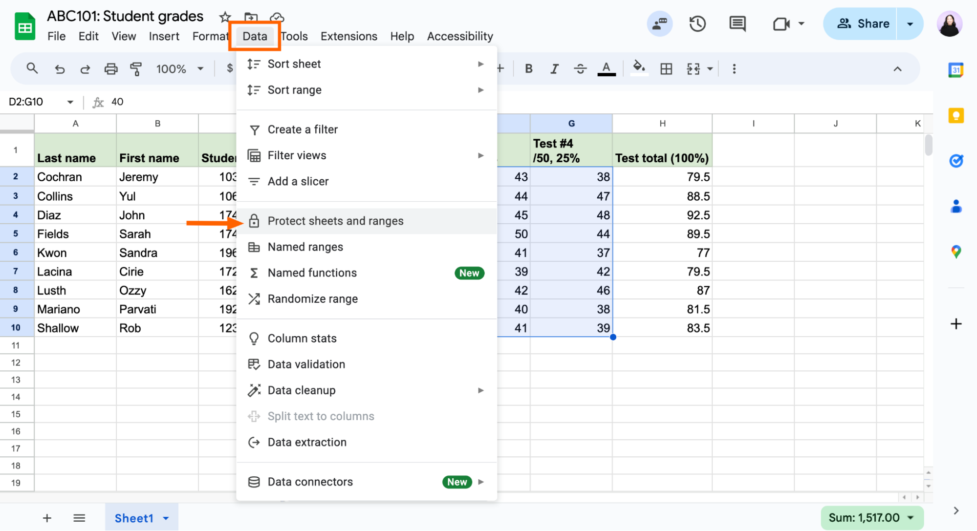
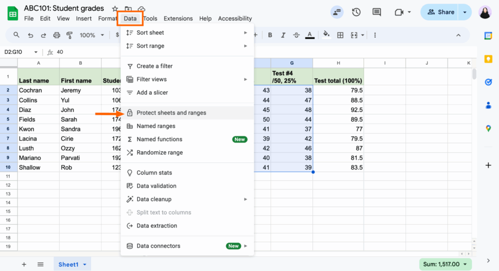
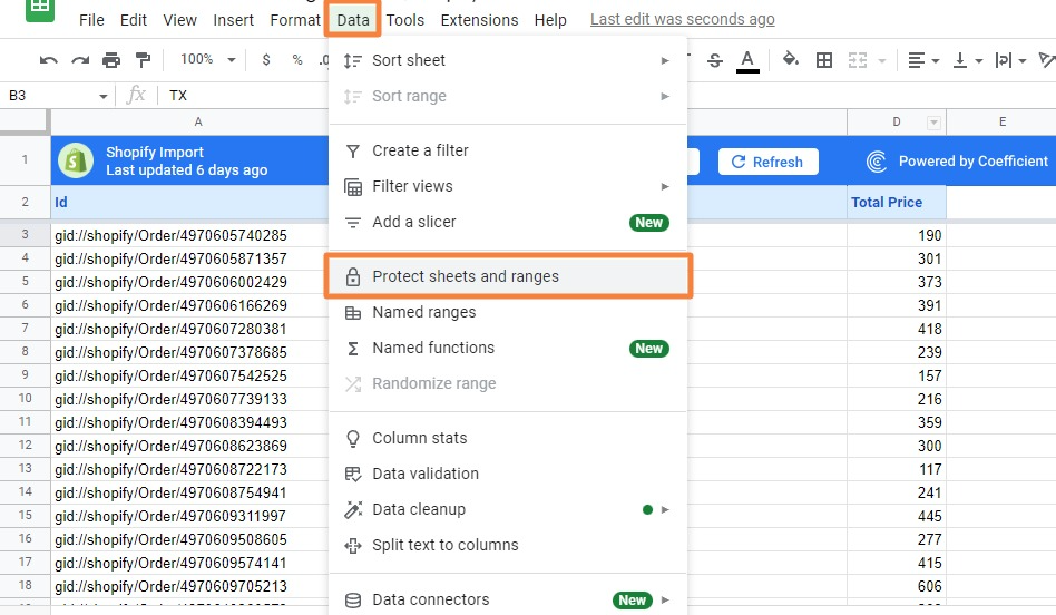
Access Protection Settings: Go to Data in the menu bar, then select Protected sheets and ranges.
Add a New Rule: A sidebar will open on the right. Click + Add a sheet or range.
Define Range/Sheet:
- The selected range will automatically populate in the Range field. You can adjust it here if needed.
- You can also choose to protect the Sheet instead of a specific range by selecting the sheet from the dropdown and checking Except certain cells if you want to leave some areas editable (similar to unlocking in Excel).
Set Permissions: Click Set permissions.
- Restrict who can edit this range:
  - Show a warning when editing this range: This is a soft protection, allowing edits but flagging them. Good for collaborative work where you want to highlight changes.
  - Restrict who can edit this range: This is the stronger protection.
    - Only you: Only your Google account can edit.
    - Custom: Specify other Google accounts or groups that can edit.
    - Copy permissions from another range: Useful for consistent protection across your spreadsheet.
      
      Example: You have a budget spreadsheet with a formula in C5 that calculates =SUM(C1:C4) for monthly expenses. You want to allow your team to input individual expense items in C1:C4 but prevent them from accidentally deleting or changing the sum formula in C5. You would select C5, go to Data > Protected sheets and ranges, add C5 as a range, and restrict editing to “Only you” or “Custom” (excluding your team members).
Click ‘Done’: Once permissions are set, click Done.

Now, anyone attempting to edit a protected cell or range without the appropriate permissions will be blocked or receive a warning, depending on your settings.

Protecting an Entire Workbook Structure

Beyond just cells and sheets, you might need to protect the actual structure of your workbook. This prevents users from adding new sheets, deleting existing ones, renaming sheets, or changing their order. This is particularly useful for complex financial models or dashboards with interdependent worksheets.

Step-by-Step: How to Protect Workbook Structure (Excel)

Open the Workbook: Make sure the workbook you want to protect is open.
Navigate to Review Tab: Go to the Review tab on the Ribbon.
Click ‘Protect Workbook’: In the Protect group, click Protect Workbook.
Choose Protection Type:
- Structure: This option prevents users from inserting, deleting, renaming, moving, or hiding sheets. This is the most common use case for workbook protection.
- Windows: (Less common now) This option protects the size and position of workbook windows when the workbook is opened.
Set Password (Optional but Recommended): Enter a Password (optional). Again, if you don’t set a password, anyone can unprotect the workbook structure.
Click OK: Confirm the password if you set one.

Now, if someone tries to right-click on a sheet tab, options like Insert, Delete, Rename, Move or Copy, and Hide will be grayed out and inaccessible. This significantly enhances the integrity of multi-sheet workbooks.

Advanced Protection Strategies and Considerations

While the basic steps cover most needs, let’s explore some more advanced scenarios and nuances.

Protecting Formulas While Displaying Results

This is a common requirement: users need to see the result of a calculation but not the formula itself, often to prevent intellectual property theft or accidental changes.

Unlock Editable Cells First: As always, identify and unlock the cells where users can enter data.
Select Cells with Formulas: Select the cells or ranges containing the formulas you want to protect and hide.
Format Cells (Excel):
- Right-click, Format Cells…, go to the Protection tab.
- Ensure Locked is checked (it is by default).
- Check the Hidden box.
Apply Sheet Protection: Go to Review > Protect Sheet (Excel) or Data > Protected sheets and ranges (Google Sheets). Set a password and define permissions.

Now, when the sheet is protected, users will see the calculated value in the cell, but the formula bar will be empty, hiding the underlying formula.

Allowing Specific Actions on a Protected Sheet

The “Allow users of this worksheet to:” section in Excel’s Protect Sheet dialog is incredibly powerful. Let’s say you have a data table with rows and columns of sales figures, and a pivot table connected to it. You want to protect the data source from direct edits but allow users to refresh or interact with the pivot table.

You would protect the sheet, uncheck Select locked cells, but check Use PivotTable reports. This ensures users can’t mess with your raw data, but they can still generate their own views and analyses from the pivot table. Similarly, if your sheet has filters, check Use AutoFilter.

Differentiating Permissions (Google Sheets)

Google Sheets excels here. You can protect a range A1:B10 allowing only “Finance Team” to edit, while range C1:D10 allows “Sales Team” to edit, and range E1:E10 is editable only by “You.” This granular control is invaluable for collaborative environments.

Unprotecting Your Data

Knowing how to protect is just half the battle; you also need to know how to reverse it when necessary.

Unprotecting a Sheet (Excel)

Navigate to Review Tab: Go to the Review tab.
Click ‘Unprotect Sheet’: In the Protect group, click Unprotect Sheet.
Enter Password: If you set a password during protection, you’ll be prompted to enter it.
Click OK: The sheet is now fully editable.

Unprotecting a Workbook Structure (Excel)

Navigate to Review Tab: Go to the Review tab.
Click ‘Unprotect Workbook’: In the Protect group, click Unprotect Workbook.
Enter Password: If you set a password, enter it.
Click OK: The workbook structure is now editable (you can insert/delete sheets, etc.).

Managing Protected Ranges/Sheets (Google Sheets)

Go to Data Menu: Select Data > Protected sheets and ranges.
Manage Rules: The sidebar will display all existing protection rules.
Edit or Remove:
- To edit a rule, click on it in the sidebar. You can then modify the range, permissions, or add/remove users.
- To remove a rule, click the trash can icon next to the rule in the sidebar.
Click ‘Done’: After making changes, click Done.

Common Pitfalls and Troubleshooting

Even with the right steps, you might run into issues. Here are some common problems and their solutions:

“My cells are still editable after I protected the sheet!”
- Cause: You likely forgot to uncheck the “Locked” property for the cells you wanted to protect. Remember, cells are “locked” by default. If you don’t explicitly unlock the editable ones, then all cells will be locked when you apply sheet protection.
- Fix: Unprotect the sheet. Go back to the Format Cells dialog for the cells you want to be editable and uncheck “Locked.” Then, re-apply sheet protection.
“I protected my sheet, but I can’t filter/sort my data anymore!”
- Cause: When you protect a sheet in Excel, common actions like sorting and filtering are disabled by default.
- Fix: Unprotect the sheet. When you re-apply Protect Sheet, make sure to check the boxes next to Use AutoFilter and/or Sort in the “Allow users of this worksheet to:” section.
“I hid my formulas, but they’re still visible in the formula bar.”
- Cause: You checked Hidden in the Format Cells dialog but forgot to actually apply Sheet Protection. The “Hidden” property only takes effect when the sheet is protected.
- Fix: Ensure you’ve completed the Protect Sheet step after setting the “Hidden” property.
“I can’t delete/rename a sheet!”
- Cause: The workbook structure is protected.
- Fix: Go to Review > Unprotect Workbook and enter the password if required.
“My Google Sheet warning message isn’t strong enough, people are still editing.”
- Cause: You likely selected “Show a warning when editing this range” instead of “Restrict who can edit this range” when setting permissions.
- Fix: Go to Data > Protected sheets and ranges, edit the rule, and choose the stronger “Restrict who can edit this range” option with appropriate user restrictions.
Lost Password: This is the most critical pitfall. If you protect a sheet or workbook with a password and then forget it, there’s no official “reset” or “recovery” method. While there are third-party tools that claim to remove Excel passwords, they are not always reliable and can be risky.
- Prevention: Always use memorable passwords. For crucial documents, consider keeping a secure record of your passwords.

Conclusion: Safeguarding Your Spreadsheet Investments

In today’s data-driven world, your spreadsheets are valuable assets. They contain critical calculations, strategic plans, and essential records. Knowing how to lock cells, ranges, and sheets to protect your data isn’t just a technical skill; it’s a fundamental aspect of data governance and security.

By following the step-by-step instructions in this guide, you can confidently prevent accidental modifications, secure sensitive formulas, control data entry, and maintain the structural integrity of your workbooks. Whether you’re collaborating with colleagues, sharing reports with clients, or just protecting your own complex analyses, these protection features are your best friends. Implement them wisely, and enjoy the peace of mind that comes with knowing your data is safe and sound, ready to empower your decisions without fear of unintended changes.

Frequently Asked Questions (FAQ)

Q1: What’s the main difference between “locking cells” and “protecting a sheet”?

A1: “Locking cells” is a cell property that, by itself, does nothing. It’s like having a lock on a door but no key. “Protecting a sheet” is the action that activates these cell properties. When you protect a sheet, all cells marked as “locked” become uneditable, while cells marked as “unlocked” remain editable. You must apply sheet protection for the cell’s “locked” status to have any effect.

Q2: Can I protect specific cells with different passwords for different users?

A2: In Microsoft Excel, you can’t assign different passwords to individual cells or ranges within the same sheet. The sheet protection password applies to the entire sheet. However, you can have different sheets with different protection passwords. In Google Sheets, you can set specific editing permissions for different ranges, allowing specific Google accounts or groups to edit certain areas while others are restricted or receive warnings.

Q3: What happens if I protect a sheet with a password and then forget the password?

A3: If you forget the password to unprotect an Excel sheet or workbook, there is no built-in recovery mechanism from Microsoft. This means you will effectively be locked out from making changes to the protected elements. Always choose memorable passwords and keep a secure record of them for important files.

Q4: Does protecting my sheet prevent someone from copying my data?

A4: Protecting a sheet primarily prevents editing the data. Users can still typically select and copy the data from protected cells (unless you uncheck “Select locked cells” during sheet protection in Excel). If you want to prevent copying sensitive information, you might consider alternative methods like converting the data to an image, distributing PDFs, or using more advanced data rights management tools if available within your organization.

Q5: Is there a way to protect my spreadsheet from being opened by unauthorized users?

A5: Protecting cells, ranges, and sheets prevents editing, not opening. To prevent unauthorized users from opening the file itself, you need to set a password to open the workbook. In Excel, this is typically done via File > Info > Protect Workbook > Encrypt with Password. In Google Sheets, you manage sharing permissions to control who can access the document at all.

See more: How to Lock Cells, Ranges, and Sheets to Protect Your Data.

Discover: AskByteWise.