SUMIF vs. SUMIFS: A Clear Comparison for Smarter Spreadsheets

Tired of sifting through rows and columns, manually adding up numbers that meet specific conditions? You’re not alone. Many spreadsheet users find themselves wishing for a magic button that could quickly sum data based on criteria like “all sales from region North” or “all expenses from October.” Good news: that magic button comes in the form of two incredibly powerful Excel and Google Sheets functions: SUMIF and SUMIFS. This guide will provide a SUMIF vs. SUMIFS: A Clear Comparison, empowering you to automate your data analysis and unlock deeper insights from your spreadsheets.

At AskByteWise.com, our mission is “Making Complex Tech Simple,” and today, we’re demystifying these essential functions. As your lead content strategist, I’ve spent over a decade breaking down spreadsheet challenges, and I can assure you that once you grasp SUMIF and SUMIFS, your approach to data will transform. You’ll move from tedious manual calculations to dynamic, criteria-driven sums, making your reports more accurate and your workday more efficient. Whether you’re an office professional tracking inventory, a student managing project budgets, or anyone who uses a spreadsheet, understanding these functions is a game-changer. Let’s dive in!

What’s the Big Deal About Conditional Summing?

Imagine you have a large dataset of sales transactions. You might want to answer questions like:

• What was the total revenue from “Product A”?
• How much did “Salesperson John” sell in “Q3”?
• What’s the sum of all invoices that are “Overdue” and “Above $1,000”?

Without conditional summing functions, you’d be manually filtering, selecting, and summing – a process prone to errors and incredibly time-consuming, especially with a growing number of rows. This is where SUMIF and SUMIFS come to the rescue. They allow you to sum numbers in a range based on conditions you define, making your data analysis tasks faster, more accurate, and infinitely more flexible. These powerful tools are fundamental for anyone working with numerical data in a spreadsheet.

Understanding the SUMIF Function: Your First Step to Smart Summing

The SUMIF function is designed for situations where you need to sum values based on one single criterion. Think of it as your go-to function when you have a straightforward question about your data. For example, “What’s the total for X?” or “Sum all values where Y is true.”

SUMIF Syntax Explained

The basic syntax for SUMIF is:

=SUMIF(range, criteria, [sum_range])

Let’s break down each argument:

• range: This is the group of cells that Excel or Google Sheets will check against your criteria. It’s the column or row where your conditions are located. For instance, if you want to sum sales for a specific product, your range would be the column containing all product names. This argument is required.
• criteria: This is the condition or rule that tells the function which cells to include in the sum. It can be a number, text, a cell reference, an expression, or a logical operator. Examples include "Apples", 100, ">50", A1. This argument is also required.
• [sum_range]: This is the actual range of cells that will be summed up. Excel or Google Sheets will sum the corresponding values in this range for the rows that meet your criteria. If you omit this optional argument, the function will sum the range itself (assuming it contains numerical values). In most business scenarios, you’ll specify a sum_range.

Practical Example 1: Summing Sales by Product Category

Let’s imagine you have a sales transaction sheet with the following columns: Product Category, Product Name, and Sales Amount. You want to find the total sales for the “Electronics” category.

Column A (Product Category)	Column B (Product Name)	Column C (Sales Amount)
Electronics	Laptop	$1,200
Apparel	T-Shirt	$30
Electronics	Smartphone	$800
Home Goods	Blender	$150
Apparel	Jeans	$60
Electronics	Tablet	$450

Here’s how you’d use SUMIF:

1. Identify your data: Your data is in cells A2:C7.
2. Define your goal: Sum all sales where the Product Category is “Electronics”.
3. Determine range: The categories are in A2:A7.
4. Determine criteria: We’re looking for "Electronics".
5. Determine sum_range: The sales amounts are in C2:C7.

Now, let’s put it all together:

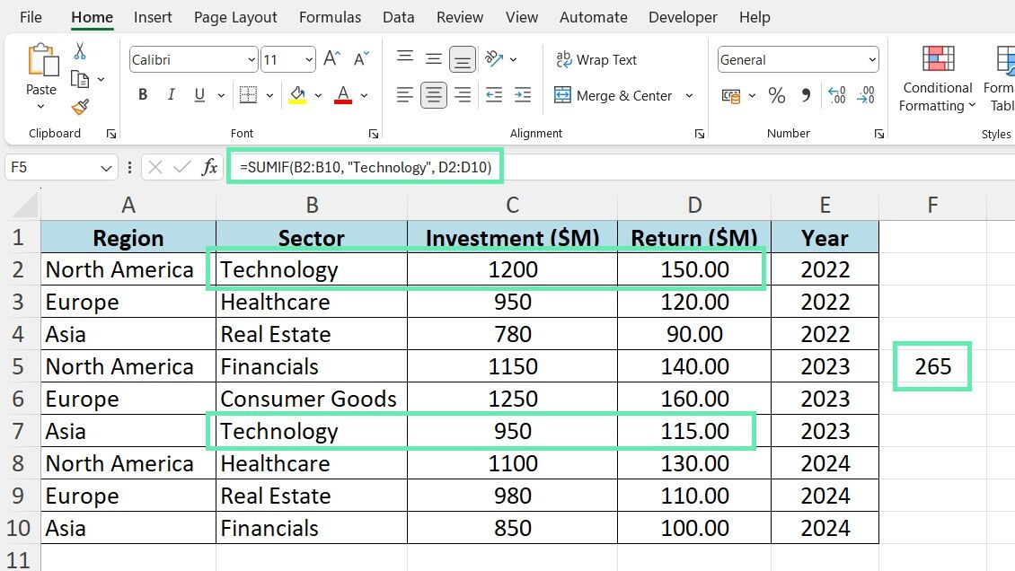
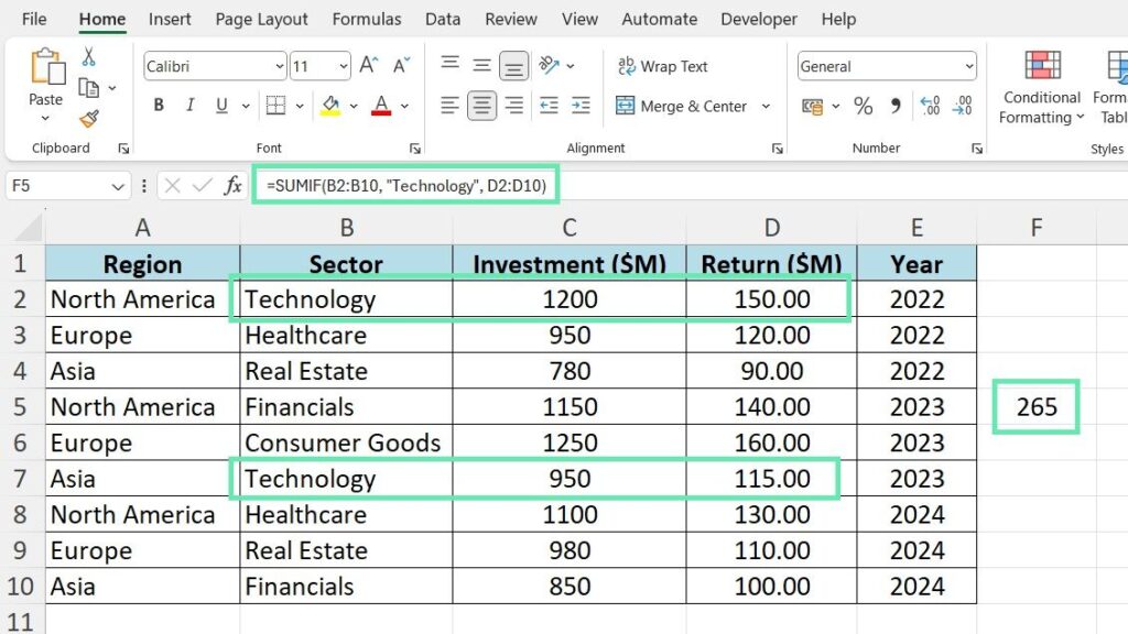
=SUMIF(A2:A7, "Electronics", C2:C7)

Explanation:

• A2:A7: The function will look in this range for matches.
• "Electronics": This is the condition. The function will find every instance of “Electronics” in the A2:A7 range.
• C2:C7: For every row where “Electronics” is found in A2:A7, the corresponding value from C2:C7 will be added to the total.

The result of this formula would be $2,450 (1200 + 800 + 450).

Tip: You can use a cell reference for your criteria instead of typing it directly into the formula. For example, if “Electronics” was in cell E1, your formula would be =SUMIF(A2:A7, E1, C2:C7). This makes your spreadsheet more flexible and easier to update!

Mastering the SUMIFS Function: When You Need More Than One Condition

While SUMIF is perfect for single conditions, real-world data often requires multiple criteria. What if you wanted to sum sales for “Product A” and only for “Region North”? Or total expenses that are “Overdue” and “Above $500”? This is precisely what the SUMIFS function is designed for. It allows you to sum values based on two or more criteria.

SUMIFS Syntax Explained

The basic syntax for SUMIFS is a bit different from SUMIF:

=SUMIFS(sum_range, criteria_range1, criteria1, [criteria_range2, criteria2], ...)

Notice the order change: sum_range comes first in SUMIFS. Let’s break it down:

• sum_range: This is the first argument in SUMIFS and it’s where the numbers you want to sum are located. This argument is required.
• criteria_range1: This is the first range that Excel or Google Sheets will check against its corresponding criteria1. It’s the column or row where your first condition is located. This argument is required.
• criteria1: This is the first condition that tells the function which cells in criteria_range1 to include in the sum. This argument is required.
• [criteria_range2, criteria2]: This is where SUMIFS really shines. You can add additional pairs of criteria_range and criteria arguments. You can include up to 127 pairs, allowing for highly specific conditional summing. These arguments are optional but are what differentiate SUMIFS from SUMIF.

Practical Example 2: Summing Sales for a Specific Product Category and Region

Let’s expand on our sales data. Now we have Product Category, Region, and Sales Amount. We want to find the total sales for the “Electronics” category only in the “West” region.

Column A (Product Category)	Column B (Region)	Column C (Sales Amount)
Electronics	East	$1,200
Apparel	West	$30
Electronics	West	$800
Home Goods	East	$150
Apparel	East	$60
Electronics	West	$450
Electronics	North	$300

Here’s how you’d use SUMIFS:

1. Identify your data: Your data is in cells A2:C8.
2. Define your goal: Sum all sales where the Product Category is “Electronics” and the Region is “West”.
3. Determine sum_range: The sales amounts are in C2:C8.
4. Determine criteria_range1 and criteria1: Categories are in A2:A8, looking for "Electronics".
5. Determine criteria_range2 and criteria2: Regions are in B2:B8, looking for "West".

Now, let’s construct the formula:

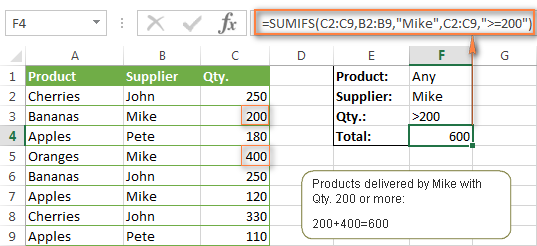
=SUMIFS(C2:C8, A2:A8, "Electronics", B2:B8, "West")

Explanation:

• C2:C8: This is the range containing the values to be summed.
• A2:A8: This is the first range to check against criteria1.
• "Electronics": This is the first condition. It will find rows where the product category is “Electronics”.
• B2:B8: This is the second range to check against criteria2.
• "West": This is the second condition. From the rows already identified as “Electronics”, it will further filter for those where the region is “West”.

The result of this formula would be $1,250 (800 + 450).

Important Note: For SUMIFS, all criteria_range arguments must have the same number of rows and columns as the sum_range. If they don’t, you’ll likely encounter a #VALUE! error. This consistency is crucial for the function to correctly map criteria to the values being summed.

SUMIF vs. SUMIFS: The Core Differences Unpacked

Now that you’ve seen both functions in action, let’s clearly outline their distinctions. Understanding these differences is key to choosing the right tool for your specific data analysis needs.

Key Distinctions

Feature	SUMIF	SUMIFS
Number of Criteria	One single criterion only.	One or more criteria (up to 127 pairs).
Syntax Order	range, criteria, [sum_range]	sum_range, criteria_range1, criteria1, …
sum_range Position	Optional, placed last. If omitted, range is summed.	Required, placed first. Cannot be omitted.
Flexibility	Simpler, less flexible.	More complex, highly flexible for multi-condition summing.
Compatibility	Available in all Excel versions.	Available in Excel 2007 and later, and Google Sheets.
Performance	Slightly faster for a single condition (marginally).	Can be slower with many criteria on very large datasets.

When to Use Which

• Use SUMIF when:

  • You need to sum values based on one specific condition.
  • Your logic is straightforward, like “total sales for this product” or “total expenses over this amount.”
  • You’re working with older versions of Excel that might not support SUMIFS.
  • You prefer a simpler, more concise formula for single conditions.

• Use SUMIFS when:

  • You need to sum values based on two or more conditions. This is where its power truly lies.
  • Your analysis requires drilling down into data with multiple filters, such as “sales of Product A by Salesperson B in Region C.”
  • You need precise control over which records are included in your sum, applying conditions across different columns.
  • You’re working with Excel 2007 or newer, or Google Sheets.

Analogy: Think of SUMIF as ordering a single-topping pizza (“Just pepperoni, please!”). SUMIFS is like building a custom pizza with multiple toppings (“Pepperoni, mushrooms, and extra cheese, but no olives!”). Both are great, but SUMIFS gives you far more customization.

Advanced Scenarios and Wildcard Characters

Beyond basic text and number matching, both SUMIF and SUMIFS offer powerful ways to refine your criteria, making them incredibly versatile data analysis tools.

Using Wildcards (*, ?, ~) with SUMIF/SUMIFS

Wildcard characters allow you to perform partial matches, which is incredibly useful when your data isn’t perfectly consistent or you need to sum based on patterns.

• *`` (Asterisk):** Represents any sequence of zero or more characters.
  • Example: "East*" would match “East”, “Eastern”, “East Coast Sales”.
  • Example: "*Shirt*" would match “T-Shirt”, “Dress Shirt”, “Shirt (Small)”.
• ? (Question Mark): Represents any single character.
  • Example: "B?ll" would match “Ball”, “Bell”, “Bill”, but not “Bull”.
  • Example: "202?” would match “2020”, “2021”, “2022”, “2023”.
• ~ (Tilde): Used as an escape character when you actually want to search for an asterisk or question mark within your data.
  • Example: "Product~*" would search for the literal string “Product*” instead of “Product” followed by any characters.

Example: Sum sales for all products that contain the word “Shirt” in their name.

Using the expanded sales data from before:

=SUMIF(B2:B8, "*Shirt*", C2:C8)

This would sum sales for any product name in column B that contains “Shirt”, regardless of what comes before or after it.

Combining with Other Functions (e.g., Dates)

When working with dates, you often need to sum data within a specific period (e.g., a month, a quarter, a year). You can use logical operators (>, <, >=, <=, <>) along with other date functions.

Example: Sum sales for “Electronics” in January 2023.

Assume you have a “Date” column (Column D) and want to sum sales for “Electronics” (Column A) within January 2023.

=SUMIFS(C2:C8, A2:A8, "Electronics", D2:D8, ">=1/1/2023", D2:D8, "<=1/31/2023")

Explanation:

• C2:C8: sum_range (Sales Amount).
• A2:A8, "Electronics": First condition (Product Category is “Electronics”).
• D2:D8, ">=1/1/2023": Second condition (Date is on or after January 1, 2023).
• D2:D8, "<=1/31/2023": Third condition (Date is on or before January 31, 2023).

Notice how we use the D2:D8 range twice with different criteria to define a date range. This demonstrates the power of SUMIFS for complex, time-based analysis.

Common Errors and How to Fix Them

Even with a clear understanding, you might run into issues. Here are some common errors and how to troubleshoot them, reinforcing your expertise as a data analyst.

1. Range Mismatch (#VALUE!)

This is a very frequent error with SUMIFS.

• Problem: The sum_range and criteria_range arguments do not have the same number of rows or columns.
• Example: =SUMIFS(C2:C10, A2:A8, "Electronics", B2:B10, "West")
  • Here, C2:C10 (9 rows) and B2:B10 (9 rows) match, but A2:A8 (7 rows) does not. This will result in a #VALUE! error.
• Fix: Ensure all ranges in your SUMIFS formula cover the exact same number of rows and columns. For example, if your data goes down to row 10, all ranges should reflect that: A2:A10, B2:B10, C2:C10.

2. Criteria Not Found (Returns 0)

If your formula returns 0 when you expect a sum, it usually means no cells met your criteria.

• Problem:
  • Typos: You’ve misspelled the criteria (e.g., "Eletronics" instead of "Electronics").
  • Case Sensitivity: While Excel is generally not case-sensitive for text criteria in SUMIF/SUMIFS, some specific scenarios or external data sources might introduce case-sensitive issues. Google Sheets is case-sensitive for exact matches.
  • Leading/Trailing Spaces: Data often contains hidden spaces that prevent an exact match. "Electronics " is not the same as "Electronics".
  • Numeric vs. Text Numbers: If your criteria_range contains numbers stored as text (e.g., '100 instead of 100), your numeric criteria might not match.
• Fix:
  • Double-check spelling: Carefully review your criteria against the actual data.
  • Use TRIM: Clean your data using the TRIM function to remove leading/trailing spaces, or manually check for them.
  • Convert data types: If numbers are stored as text, convert them to actual numbers.
  • Check for invisible characters: Use the CLEAN function or find/replace to remove non-printable characters.

3. Incorrect Quoting for Text Criteria

• Problem: Text criteria (like "Electronics") must always be enclosed in double quotation marks. Numbers and cell references typically do not need quotes (unless combined with operators, e.g., ">100").
• Fix: Make sure all your text criteria are properly quoted.
  • Correct: =SUMIF(A:A, "Electronics", C:C)
  • Incorrect: =SUMIF(A:A, Electronics, C:C) (will likely result in a #NAME? error)

4. Overlapping Ranges or Circular References

While less common, sometimes range selections can create circular reference errors or sum unintended values.

• Problem: Your sum_range overlaps with a criteria_range in a way that creates a logical loop or you accidentally include the cell containing the formula itself in one of the ranges.
• Fix: Always carefully define your ranges. Avoid including header rows or the formula cell within your data ranges. Ensure the data being summed is distinct from the data being evaluated for criteria.

Beyond SUMIF and SUMIFS: Alternative Tools

While SUMIF and SUMIFS are incredibly powerful, they are not the only ways to perform conditional summing in a spreadsheet. Depending on the complexity and your comfort level, you might explore these alternatives:

• Pivot Tables: For highly dynamic, multi-criteria summaries, Pivot Tables are unparalleled. They allow you to drag and drop fields to quickly group, count, average, and sum data based on various dimensions without writing a single formula. They are fantastic for exploratory data analysis.
• DSUM Function: The DSUM function is part of Excel’s database functions. It’s designed for more complex conditional summing, especially when your criteria are laid out in a separate range on your sheet, similar to a mini-database query. While powerful, its syntax and setup are often considered more complex than SUMIFS for most users.
• Array Formulas (with SUM and IF): Before SUMIFS was introduced, users would often combine SUM and IF in an array formula (e.g., {=SUM(IF(condition1, IF(condition2, values_to_sum)))}). While still viable, SUMIFS is generally more efficient and easier to write for multiple conditions.

For most office professionals and students, mastering SUMIF and SUMIFS will cover 90% of their conditional summing needs.

Conclusion: Empowering Your Data Analysis

Congratulations! You’ve just taken a significant leap in your spreadsheet proficiency. By understanding the nuances of SUMIF vs. SUMIFS: A Clear Comparison, you’re now equipped to tackle complex data analysis challenges with confidence and efficiency. No more manual calculations or error-prone filtering. You can now craft precise formulas that extract exactly the information you need, whether it’s total sales by a single product category or revenue generated by a specific salesperson for a particular product in a given region during a certain month.

Remember, SUMIF is your go-to for single conditions, while SUMIFS unlocks the power of multiple conditions. Practice these functions with your own data, experiment with different criteria, and don’t be afraid to make mistakes – that’s how we learn best. At AskByteWise.com, we believe that “Making Complex Tech Simple” transforms not just your skills, but your entire approach to problem-solving. Go forth and sum wisely!

Frequently Asked Questions (FAQ)

Q1: Can SUMIF or SUMIFS be used in Google Sheets?

A1: Yes, absolutely! Both SUMIF and SUMIFS functions work identically in Google Sheets as they do in Microsoft Excel. The syntax, arguments, and behavior are the same, making them cross-platform compatible for conditional summing.

Q2: Why would I use SUMIF if SUMIFS can handle multiple and single conditions?

A2: While SUMIFS can technically be used for a single condition (by just providing one criteria_range and criteria pair), SUMIF has a slightly simpler syntax, especially regarding the sum_range placement. For very basic, single-condition tasks, SUMIF might be marginally easier to write and read. However, if you anticipate needing to add more conditions later, starting with SUMIFS might save you time on refactoring the formula.

Q3: How do I make my SUMIF/SUMIFS criteria case-sensitive?

A3: By default, both Excel’s SUMIF and SUMIFS functions are not case-sensitive for text criteria. For example, “electronics” will match “Electronics”. If you need case-sensitive matching, you’ll need to use more advanced array formulas involving functions like SUMPRODUCT combined with EXACT, or other helper columns and functions. Google Sheets’ SUMIF/SUMIFS are case-sensitive for exact text matches by default.

Q4: Can I use SUMIF or SUMIFS with external data (e.g., from another workbook)?

A4: Yes, you can reference ranges in other worksheets within the same workbook, or even ranges in entirely different workbooks (provided those workbooks are open or the path is correctly specified). The syntax for referencing external data typically involves the sheet name (e.g., Sheet2!A:A) or the workbook and sheet name (e.g., '[Sales Data.xlsx]Sheet1'!A:A).

Q5: What’s the main performance consideration between SUMIF and SUMIFS on large datasets?

A5: On extremely large datasets (hundreds of thousands of rows or more), SUMIFS can sometimes be slightly slower than SUMIF due to the overhead of evaluating multiple conditions. However, for typical datasets found in everyday business operations (up to tens of thousands of rows), the performance difference is usually negligible. The most significant performance impact often comes from using entire column references (e.g., A:A) in large spreadsheets, which forces the function to evaluate many unnecessary blank cells. It’s generally better to limit your ranges to the actual data area (e.g., A2:A10000).

See more: SUMIF vs. SUMIFS: A Clear Comparison.

Discover: AskByteWise.