How to Create a Dropdown List with Data Validation in Spreadsheets

Are you tired of sifting through messy data, correcting typos, and dealing with inconsistent entries in your spreadsheets? Imagine a world where every piece of data is entered correctly, uniformly, and with minimal effort. As Noah Evans, lead content strategist at AskByteWise.com, I’ve spent over a decade helping professionals like you conquer spreadsheet challenges. Today, we’re diving into a powerful tool that makes this vision a reality: the dropdown list with data validation. This definitive guide will show you how to create a dropdown list with data validation, transforming your spreadsheets from a source of frustration into a beacon of efficiency and accuracy. Get ready to streamline your data entry, boost data integrity, and impress your colleagues!

Why Use Dropdown Lists with Data Validation?

In the fast-paced world of business and academia, accurate data is the bedrock of sound decisions. Whether you’re tracking project statuses, categorizing inventory, or managing student assignments, manual data entry is a common culprit behind errors, inconsistencies, and ultimately, wasted time.

Dropdown lists, powered by data validation, act as your data’s gatekeeper. Instead of allowing users to type anything into a cell, you provide a pre-defined set of options. This simple yet incredibly effective technique offers several critical benefits:

• Ensures Data Integrity: By restricting entries to a specific list, you eliminate typos, variations in spelling (e.g., “NY” vs. “New York”), and incorrect data formats. This means cleaner data for analysis and reporting.
• Speeds Up Data Entry: Users can simply select an option from a list, which is much faster than typing, especially for frequently used categories. This drastically improves user experience.
• Reduces Errors: Fewer manual inputs mean fewer mistakes. This saves valuable time that would otherwise be spent on error correction.
• Improves User Experience: Clear, pre-defined options guide users, making your spreadsheets more intuitive and user-friendly, especially for those who might not be familiar with the data’s specific requirements.
• Facilitates Data Analysis: Consistent data makes it easier to use spreadsheet functions like COUNTIF, SUMIF, VLOOKUP, or create pivot tables without having to clean up inconsistent entries first.

Consider a scenario where you’re managing a sales pipeline. Instead of allowing sales representatives to type “Pending,” “In Progress,” “Closed Won,” “Closed Lost,” or even “Awaiting Decision” into a status column, a dropdown list ensures they choose from a standardized set of options. This consistency is invaluable for generating accurate reports on conversion rates or pipeline velocity.

Getting Started: The Basics of Data Validation

Before we dive into creating dropdowns, let’s understand what data validation is. Data validation is an Excel (and Google Sheets) feature that allows you to define rules for what can be entered into a cell. These rules can include limiting data to whole numbers, dates, text length, or, as in our case, a predefined list of items.

You’ll find the Data Validation feature under the Data tab in the Excel ribbon. In Google Sheets, it’s also under the Data menu. This powerful feature is your first line of defense against erroneous data.

Now, let’s roll up our sleeves and create our first dropdown list!

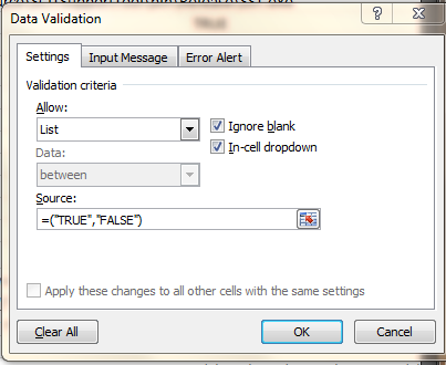
Method 1: Creating a Simple Dropdown List from a List of Items

This method is perfect for short, static lists where the options are unlikely to change often. Think of lists like “Yes, No, N/A” or “High, Medium, Low.”

Step-by-Step Guide

1. Select the Target Cell(s): Click on the cell or drag to select the range of cells where you want your dropdown list to appear. For instance, if you want a dropdown in cell B2, select B2. If you want it in B2:B10, select that entire range.

2. Access Data Validation: Go to the Data tab in the Excel ribbon. In the Data Tools group, click on Data Validation.

3. Configure Settings: The Data Validation dialog box will appear.

   • Navigate to the Settings tab.
   • Under Allow:, click the dropdown arrow and select List.
   • In the Source: field, type your list items, separated by commas. For example, if you’re listing project priorities, you might type: High,Medium,Low,Critical.

4. Confirm and Apply: Click OK.

You’ll now see a small dropdown arrow next to your selected cell(s). Click the arrow, and your list of options will appear, ready for selection!

Tip: This method is quick and easy, but less flexible. If your list of items frequently changes, you’ll have to manually update the Source field in every data validation rule. For more dynamic lists, the next method is far superior.

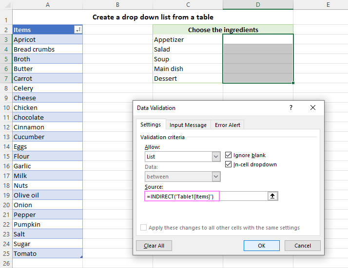
Method 2: Creating a Dropdown List from a Range of Cells (Recommended)

This is the most common and highly recommended method for creating dropdown lists, especially when your list of options is long, might change, or needs to be managed separately. By linking your dropdown to a range of cells, any updates to that range will automatically reflect in your dropdowns.

Let’s imagine you’re managing product categories for an e-commerce site. Your categories might include “Electronics,” “Apparel,” “Home Goods,” “Books,” “Sports,” etc. These might expand over time.

Step-by-Step Guide

1. Create Your Source List:

   • It’s best practice to create your list of options on a separate sheet within your workbook or in a dedicated column that won’t be accidentally edited or deleted. Let’s say you create a new sheet called “Lists” and type your product categories into cells A1:A5.
     • A1: Electronics
     • A2: Apparel
     • A3: Home Goods
     • A4: Books
     • A5: Sports

2. Select the Target Cell(s): Go back to the sheet where you want the dropdown (e.g., your “Sales Data” sheet) and select the cell or range (e.g., C2:C10) where you want the dropdowns to appear.

3. Access Data Validation: Go to the Data tab > Data Validation.

4. Configure Settings:

   • In the Data Validation dialog box, go to the Settings tab.
   • Under Allow:, select List.
   • In the Source: field, instead of typing values, click the small up-arrow icon (it looks like a mini spreadsheet icon) to the right of the field. This will allow you to select a range.
   • Navigate to your “Lists” sheet and select the range A1:A5 (or whatever range contains your options). Excel will automatically populate the Source: field with the correct reference, e.g., =Lists!$A$1:$A$5.
   • Alternatively, you can manually type the range reference directly into the Source: field: =Lists!A1:A5.

5. Confirm and Apply: Click OK.

Now, your dropdowns are linked to the range on your “Lists” sheet. If you add “Automotive” to cell A6 on your “Lists” sheet, your dropdowns will automatically include it (as long as your source range in data validation was defined to include A6 or beyond, or if you make your Named Range dynamic, which we’ll cover later).

Important Note: When defining the source range, ensure it covers all potential future additions to your list. A common mistake is to select only the currently populated cells. Selecting a slightly larger range than currently needed (e.g., A1:A100 if you only have 5 items) allows for future expansion without re-editing the data validation rule.

Method 3: Enhancing Dropdowns with Named Ranges (For Clarity & Robustness)

While Method 2 is excellent, using Named Ranges takes it a step further in terms of clarity, manageability, and robustness. A Named Range is simply a user-defined name given to a cell or range of cells. Instead of referring to Lists!$A$1:$A$5, you can refer to ProductCategories. This makes your formulas and data validation rules much easier to understand and manage.

What are Named Ranges?

Imagine you have a complex spreadsheet with many different lists: product categories, employee departments, project stages, sales regions. Instead of memorizing which sheet and range each list occupies (e.g., Sheet2!D1:D15), you can give each of them a meaningful name like DeptList or Regions. This not only makes your spreadsheet easier to navigate but also enhances readability, especially when working with more complex formulas or functions.

Creating a Named Range for Your List

Let’s continue with our product categories example (Electronics, Apparel, Home Goods, Books, Sports) located in Lists!A1:A5.

1. Select Your Source Range: Navigate to your “Lists” sheet and select the range A1:A5.

2. Open the New Name Dialog: Go to the Formulas tab in the Excel ribbon. In the Defined Names group, click on Define Name.

3. Define the Name: The New Name dialog box will appear.

   • In the Name: field, type a clear, descriptive name for your range. For our example, let’s use ProductCategories. (Names cannot contain spaces, so use underscores or camelCase).
   • The Scope: typically defaults to Workbook, which is usually what you want, meaning the name is recognized anywhere in your entire workbook.
   • The Refers to: field should already be populated with your selected range (e.g., =Lists!$A$1:$A$5).

   

4. Confirm and Apply: Click OK.

You’ve now successfully created a Named Range! You can view and manage all your Named Ranges by clicking Name Manager in the Formulas tab.

Using a Named Range in Data Validation

Now, let’s connect our newly created Named Range to our dropdown list.

1. Select the Target Cell(s): Go back to your “Sales Data” sheet and select the cell or range (e.g., C2:C10) where you want the dropdowns.

2. Access Data Validation: Go to the Data tab > Data Validation.

3. Configure Settings:

   • In the Data Validation dialog box, go to the Settings tab.
   • Under Allow:, select List.
   • In the Source: field, type an equals sign (=) followed by your Named Range. In our example: =ProductCategories.

4. Confirm and Apply: Click OK.

Your dropdowns now use the ProductCategories Named Range as their source. This is incredibly powerful. If you later need to add a new category or change an existing one, you only need to update your source range on the “Lists” sheet (and potentially adjust the Named Range‘s “Refers to” if the list expands beyond its initial definition, though advanced users can make Named Ranges dynamically sized using formulas like OFFSET or INDIRECT).

Adding Input Messages and Error Alerts (Improving User Experience)

Dropdown lists are great, but what happens if a user is unsure what to select, or if they accidentally try to type something that isn’t on the list? This is where Input Messages and Error Alerts come in, significantly improving the user experience and ensuring robust data integrity.

Input Message: Guiding Your Users

An Input Message appears when a user selects a cell with data validation, providing instructions or context before they even try to enter data. It’s like a friendly tooltip.

1. Access Data Validation: Select your dropdown cell(s), then go to Data tab > Data Validation.

2. Configure Input Message:

   • Go to the Input Message tab.
   • Check the box for Show input message when cell is selected.
   • In the Title: field, enter a brief, descriptive title (e.g., Select Category).
   • In the Input message: field, provide clear instructions (e.g., Please choose a product category from the dropdown list.).

3. Confirm and Apply: Click OK.

Now, when a user clicks on one of your dropdown cells, a small message box will appear, guiding them on what to do.

Error Alert: Preventing Invalid Entries

An Error Alert pops up if a user attempts to enter data that doesn’t conform to your validation rules (i.e., typing something not in the dropdown list). You have three styles of alerts:

• Stop: This is the strictest. It prevents users from entering invalid data and forces them to correct it or cancel. This is typically what you want for critical data.
• Warning: This allows users to enter invalid data but warns them about it first. They can choose to proceed with the invalid entry or go back and correct it.
• Information: This is the most lenient. It simply informs the user that the data is invalid but allows them to proceed without any further prompts.

Let’s set up a “Stop” error alert for maximum data integrity.

1. Access Data Validation: Select your dropdown cell(s), then go to Data tab > Data Validation.

2. Configure Error Alert:

   • Go to the Error Alert tab.
   • Check the box for Show error alert after invalid data is entered.
   • In the Style: dropdown, select Stop.
   • In the Title: field, enter an alert title (e.g., Invalid Entry).
   • In the Error message: field, provide a helpful message (e.g., The value you entered is not in the allowed list. Please select an option from the dropdown or cancel.).

   

3. Confirm and Apply: Click OK.

Now, if someone tries to type “Gadgets” into your product category column, they will be met with a Stop alert, preventing the invalid data from being committed. This is crucial for maintaining a clean and accurate column of data.

Analogy: Think of data validation as a bouncer at a club. The Input Message is the sign outside explaining the dress code. The Error Alert is the bouncer stopping someone at the door if they don’t meet the requirements, either politely asking them to change (Warning/Information) or flat-out denying entry until they comply (Stop).

Handling Common Issues with Dropdown Lists

Even with the best planning, you might encounter a few hiccups. Here’s how to troubleshoot common problems:

1. Dropdown Arrow Not Appearing

• Check Data Validation Settings: Select the cell and go to Data > Data Validation. Ensure that Allow: is set to List and that the Source: field contains a valid list or Named Range.
• “In-cell dropdown” checkbox: On the Settings tab of the Data Validation dialog, make sure the In-cell dropdown checkbox is selected. If it’s unchecked, the arrow won’t appear.

2. Invalid Data Still Being Entered

• Error Alert Style: Double-check your Error Alert settings (Data Validation > Error Alert tab). If it’s set to Warning or Information, the user can override the alert. For strict prevention, always choose Stop.
• Existing Invalid Data: Data validation only applies to new entries or edited cells. If a cell already contained invalid data before you applied data validation, that data won’t be flagged.
  • To find existing invalid data, select the range where you applied data validation, go to Data > Data Validation, and click Circle Invalid Data. Excel will highlight any cells that don’t meet the validation rule.
• Copy-Pasting Issues: If users are copy-pasting values from other cells or external sources, they might bypass the dropdown. Data validation rules are copied with the cell formatting, but if they paste a value over the cell without retaining the validation, it could become invalid.
  • Solution: Educate users, or use Paste Special > Validation if you want to apply validation to cells that have been cleared or pasted over.

3. List Source Not Updating Automatically

• Source Range Definition: If you’re using Method 2 (range of cells) and your list expands, you need to ensure your Data Validation Source range (e.g., =$A$1:$A$5) has been updated to include the new rows (e.g., =$A$1:$A$10).
• Named Range (Manual Update): If you’re using a Named Range, and your source list expands, you’ll need to update the Refers to: property of that Named Range via the Formulas > Name Manager.
• Dynamic Named Ranges (Advanced): For a truly dynamic list that automatically adjusts as you add or remove items from your source, you can define your Named Range using formulas like OFFSET or INDIRECT combined with COUNTA. This is an advanced technique, but it’s incredibly powerful for lists that frequently change size. For example, in Excel, you might define a Named Range as =OFFSET(Lists!$A$1,0,0,COUNTA(Lists!$A:$A),1). This formula automatically resizes the range based on the number of non-empty cells in column A of the “Lists” sheet.

4. Copying and Pasting Data Validation

• Using the Format Painter: The easiest way to apply existing data validation to other cells is to use the Format Painter. Select a cell with the desired validation, click the Format Painter icon (on the Home tab), then click or drag over the cells where you want to apply it.
• Paste Special > Validation: Alternatively, copy a cell with data validation, select the target cell(s), right-click, choose Paste Special, and then select Validation.

Google Sheets Specifics (Briefly)

While the core concepts of how to create a dropdown list with data validation are identical across Excel and Google Sheets, the interface and some features might differ slightly.

• Accessing Data Validation: In Google Sheets, you select your cell(s), then go to Data > Data validation.
• Setting Up Rules: The dialog box is straightforward. You choose “List from a range” or “List of items” and define your source.
• Input Messages & Error Alerts: Google Sheets combines the input message into the rule definition, often appearing as “Help Text” or “Show validation help text.” The error alert is typically managed by checking “Reject input” (similar to Excel’s “Stop” style) or “Show warning” (similar to “Warning” style).
• Named Ranges: Google Sheets also supports Named Ranges (Data > Named ranges), and they function similarly to Excel, making your data validation rules cleaner.
• Dynamic Dropdowns: For dynamic lists in Google Sheets, the INDIRECT function within a Named Range is commonly used, often with COUNTA or FILTER to create auto-expanding lists.

Conclusion: Master Your Data Entry

Congratulations! You’ve learned how to create a dropdown list with data validation using multiple methods, enhanced them with user-friendly messages and error alerts, and even explored how to troubleshoot common issues. By implementing these techniques, you’re not just creating a dropdown; you’re building a robust, error-resistant data entry system that saves time, ensures accuracy, and makes your spreadsheets genuinely reliable.

From standardizing product categories for a sprawling inventory list to managing the status of projects in a large organization, dropdown lists are an indispensable tool for any spreadsheet user. They elevate your data, making it easier to analyze, report on, and trust.

Remember, practice makes perfect. Experiment with different lists, apply the various methods, and leverage the input messages and error alerts to craft spreadsheets that are intuitive and foolproof. Keep asking questions, keep exploring, and keep Making Complex Tech Simple!

Frequently Asked Questions (FAQ)

Q1: Can I create a dependent dropdown list, where the options in one dropdown change based on the selection in another?

A: Yes, absolutely! This is an advanced but incredibly useful technique often referred to as a “dependent” or “cascading” dropdown list. It typically involves using Named Ranges in conjunction with formulas like INDIRECT in Excel or FILTER in Google Sheets to dynamically change the source list for the second dropdown based on the value selected in the first. It’s a fantastic way to guide users through multi-level selections (e.g., selecting a country, then only seeing cities within that country). While powerful, it’s a bit more complex than the methods covered in this introductory tutorial and often warrants its own dedicated guide.

Q2: How do I remove a dropdown list from a cell or range of cells?

A: Removing a dropdown list is just as easy as creating one.

1. Select the cell or range from which you want to remove the dropdown.
2. Go to the Data tab > Data Validation.
3. In the Data Validation dialog box, click the Clear All button (usually at the bottom left).
4. Click OK.
   This will remove the data validation rule and the dropdown arrow, allowing any data to be entered into those cells again.

Q3: My list source is on another sheet. Is that okay, or should it be on the same sheet as the dropdown?

A: It’s not only okay but often considered best practice to keep your list sources on a separate, dedicated sheet (e.g., named “Lists,” “Lookup Data,” or “Admin”). This helps keep your main data sheets clean and uncluttered, reduces the risk of accidental modification of your source lists, and makes your workbook more organized and professional. Just ensure the sheet with your source list isn’t hidden in a way that makes it difficult to manage.

Q4: Can I add a blank option to my dropdown list?

A: Yes! A blank option is often desirable to indicate “no selection” or to allow a cell to be cleared. You can add a blank option in two main ways:

1. If using a comma-separated list (Method 1): Simply include a blank space or an empty string between commas in your Source field, like High,Medium, ,Low.
2. If using a range of cells (Method 2 or 3): Just include a blank cell at the top of your source range. For instance, if your list is in A1:A5, leave A1 empty and start your actual options from A2. The blank cell will then appear as a selectable option in your dropdown.

Q5: What’s the difference between “Stop,” “Warning,” and “Information” for Error Alerts?

A: These three styles dictate how Excel responds when a user enters invalid data into a cell with data validation:

• Stop: This is the most restrictive. It prevents the user from entering invalid data. An error message appears, and the user must either correct the entry to a valid option or cancel the entry entirely.
• Warning: This is less restrictive. An error message appears, but it gives the user three choices: Yes (to accept the invalid data), No (to edit the invalid data), or Cancel (to remove the invalid data). The user can override the validation if they choose.
• Information: This is the least restrictive. An informational message appears, simply notifying the user that the data is invalid. The user can then click OK to accept the invalid data or Cancel to remove it. It offers no real barrier to entering incorrect data but serves as a gentle reminder.

For ensuring data integrity, Stop is almost always the recommended style for critical data entry.

See more: How to Create a Dropdown List with Data Validation.

Discover: AskByteWise.